Chapter 12 Sensitivity to mispronunciations
For the mispronunciation trials, there is no correct “target”, as there is for the other conditions. The design of the task allows the child to associate a mispronunciation with an unfamiliar object or with the familiar object with a name that sounds like the mispronunciation. As a result, I analyzed the mispronunciation trials separately for both initial-fixation locations. One analysis handled trials where a child’s gaze started on the familiar object and another analysis handled trials starting on the unfamiliar object. For these models, I fit a Bayesian logistic regression growth curve model that included indicators for age and time × age interactions, as in the model from Chapter 5. The linear model was therefore:
\[ \small \begin{align*} \text{log\,odds}(\text{looking}) =\ &\beta_0 + \beta_1\text{Time}^1 + \beta_2\text{Time}^2 + \beta_3\text{Time}^3\ + &\text{[age 3 growth curve]} \\ (&\gamma_{0} + \gamma_{1}\text{Time}^1 + \gamma_{2}\text{Time}^2 + \gamma_{3}\text{Time}^3)*\text{Age\,4}\ + \ &\text{[age 4 adjustments]} \\ (&\delta_{0} + \delta_{1}\text{Time}^1 + \delta_{2}\text{Time}^2 + \delta_{3}\text{Time}^3)*\text{Age\,5} \ &\text{[age 5 adjustments]} \\ \end{align*} \normalsize \]
The mixed effects model included by-child and by-child-by-age random effects so that it would capture how a child’s growth curve features may be similar over developmental time (by-child effects) and may differ at each age (by-child-by-age effects). Appendix D contains the R code used to fit these models along with a description of the model’s specification/syntax.
For these analyses, I modeled the data from 300 to 1500 ms after target onset. As in the real word vs. nonword analyses, I removed any age × child levels if the child’s data had fewer than 4 fixations in a single time bin. As a result, children had to have at least 4 looks to one of the two images in every 50-ms time bin. For the unfamiliar-initial trials, this screening removed 6 children at age 3, 6 at age 4, and 2 at age 5, and for the familiar-initial trials, this screening removed 1, 4, and 0 children at ages 3, 4, and 5, respectively.
12.1 Unfamiliar-initial trials: Move along now
When preschoolers started on the image of a novel object and heard a mispronunciation, they looked to the familiar image. Figure 12.1 shows the average of children’s growth curves along with the 100 model-estimated group averages. The growth curves all cross the .5 threshold, so the children on average looked more to the familiar than the unfamiliar image. Granted, the degree of referent selection is not as strong as that observed for the real words or nonwords. For those conditions, the average growth curve reached a peak of around .77 at age 3, but for the mispronunciations the age-3 peak is around .62. Children also were comparatively slower to process mispronunciations. For the real-word condition, the average age-3 growth curve crosses .5 looking probability around 775 ms after target onset, whereas in the mispronunciation condition, this threshold is crossed at 1000 ms. Children associate the mispronunciation with the familiar object, although they are slower and show greater uncertainty compared to real word trials.
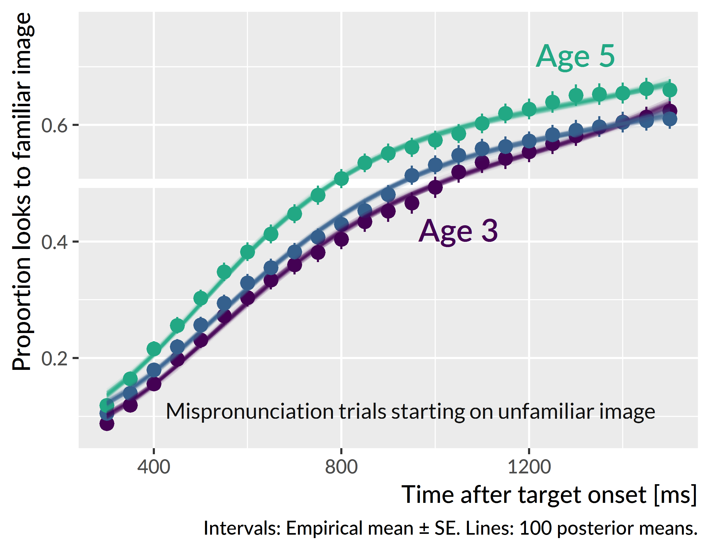
Figure 12.1: Average looks to the familiar image for mispronunciation trials starting on the unfamiliar image at each age. Lines represent 100 posterior predictions of the group average (the average of participants’ individually predicted growth curves).
Of the growth curve features, developmental changes were only observed for the average probability (intercept) and peak probability features. At age 3, the average proportion of looks to the familiar image was .37 [90% UI: .34, .40]. At age 4, the looking proportion increased by .04 [−.01, .08] to .40 [.37, .44]. This year-over-year change was probably positive, but the uncertainty interval still includes a change of 0 as a plausible result. Visually, this uncertainty appears in the growth curve plot by how close together the age-3 and age-4 growth curves appear. At age 4, the average proportion of looks increased by .07 [.03, .12] to .48 [.45, .51]. Here, there is more certainty that the year-over-year change was positive, and this result is consistent with the visual separation of the age-5 growth curve from the others. In short, performance was similar for age 3 and age 4 but there was a marked improvement at age 5.
Figure 12.2 shows participant’s growth curve peaks for each year of the study. The peaks were computed as in other chapters by taking the median of the five highest values on the curve. The average of the participants’ peak looking probabilities followed the same pattern as the average looking probabilities: similar levels at age 3 and age 4 (.63 versus .64) but a clear gain in looking peak probability at age 5 (.69).
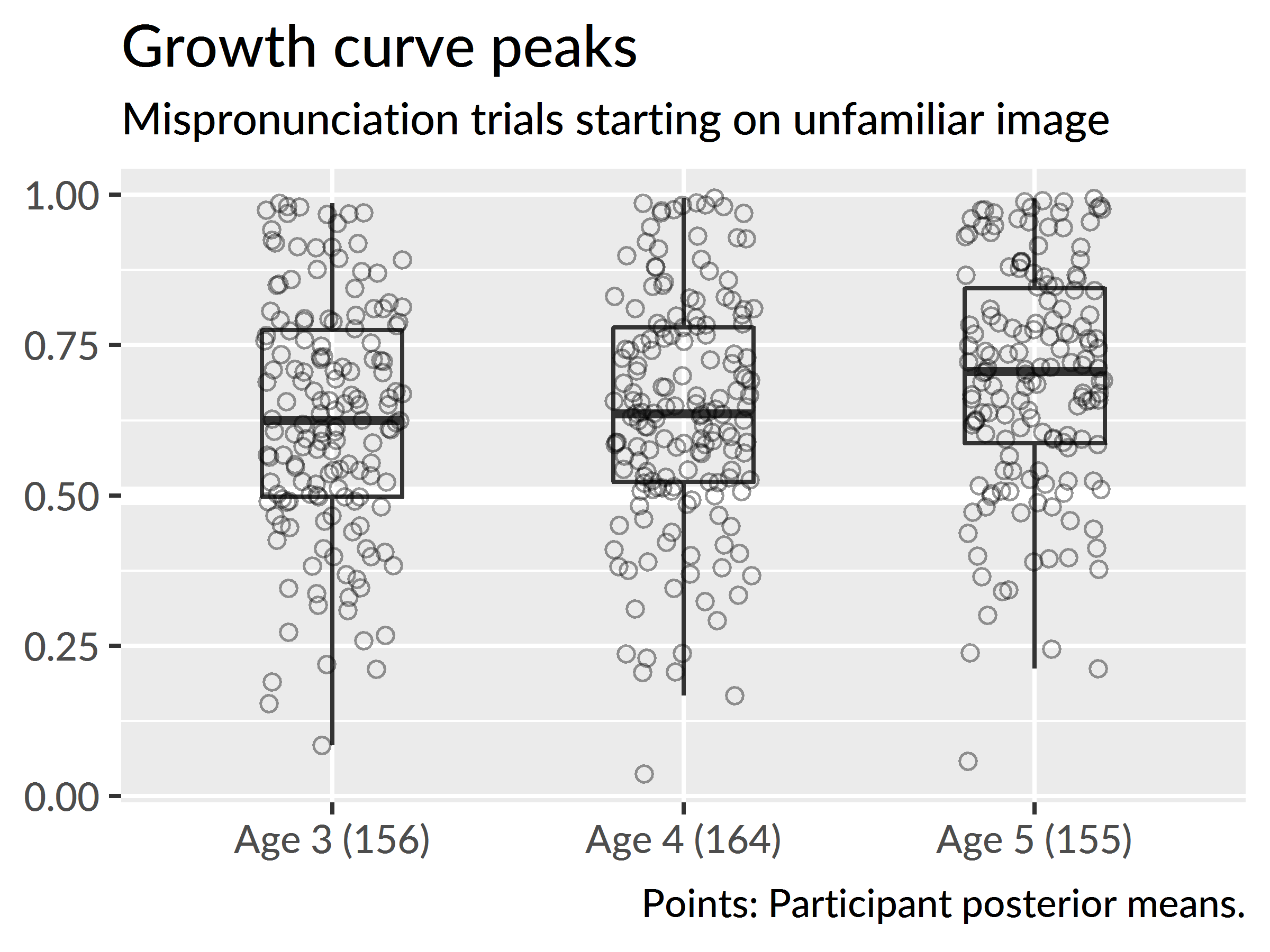
Figure 12.2: Growth curve peaks by age for mispronunciation trials starting on the unfamiliar image.
Figure 12.2 also indicates how most of the children at each age favored the familiar object over the unfamiliar object. The bottom hinge of the boxplots mark the location of the 25th percentile. Therefore, approximately 75% of children at age 3 were on or above the .5 threshold. Unlike the other conditions, very few listeners achieve a peak of looking probability of .99: At age 5, only 3 [1, 5] children reached ceiling performance, compared to approximately 40 for nonwords and 13 for real words.
None of the other growth curve features showed developmental changes. That is, there were no credible year-over-year changes for the linear, quadratic or cubic time components of the growth curve. Although Figure 12.1 shows children’s probability of looking to the familiar image increasing more quickly at age 5, this effect cannot be clearly tied to any of the model’s polynomial time features. After 600 ms, the age-5 curve is almost parallel to other curves. This visual feature is consistent with the intercept effect: The curve is higher than the others on average, but it does not show any differences in shape.
12.1.1 Child-level predictors
I tested whether child-level measures predicted looking behavior under these conditions. First, I asked if performance on a minimal pair discrimination task at age 3 predicted looking behavior at age 3. The rationale here is the hypothesis that children with better minimal pair discrimination may be especially sensitive to mispronunciations. Proportion of items correct on the task did not correlate with growth curve peaks, r = −.03 [90% UI: −.05, −.01], n = 138, nor with any other growth curve measures.
I also tested whether expressive vocabulary (EVT-2 standard score) predicted performance in this condition. In this case, there were significant effects at age 3 where a higher expressive vocabulary predicted higher peak probabilities and higher average probabilities. These effects, however, were very small. As shown in Figure 12.3, for example, a 15-point increase in expressive vocabulary predicted an increase of growth curve peak of .03, R2 = .03. Expressive vocabulary did not predict any of the growth curve features at age 4 or at age 5.
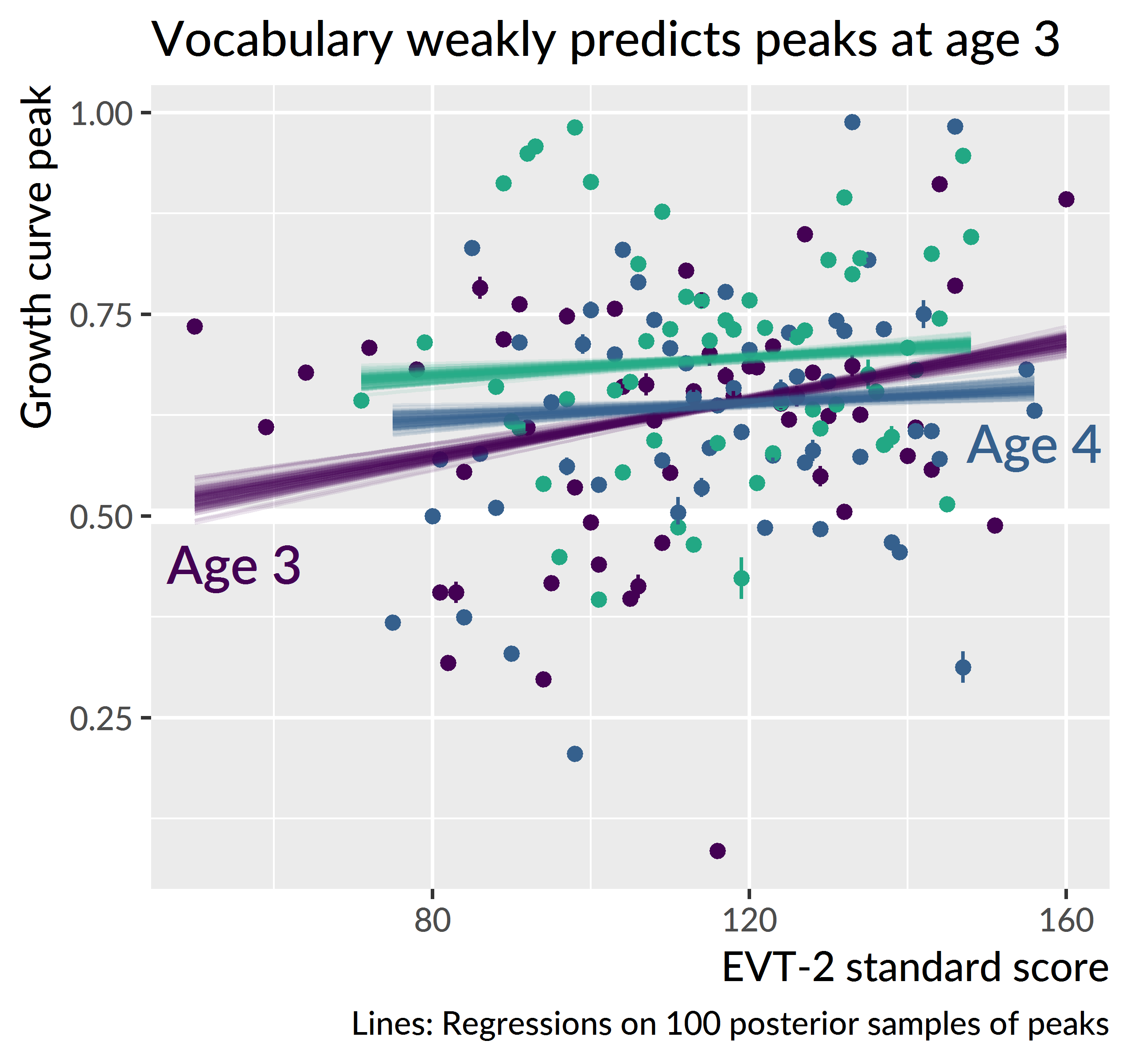
Figure 12.3: Relationship between expressive vocabulary and growth curve peaks for mispronunciation trials starting on the unfamiliar image. I took 100 draws from the posterior distribution and computed participants’ growth curve peaks for each draw. Points represent the mean and standard error of 100 peaks. Lines represent regressions fit for each draw.
Summary. When children are looking at the unfamiliar object and hear a mispronunciation, they shift their looks on average to the familiar image that sounds like the mispronunciation. Children are much more uncertain in this condition, compared to the real-word and nonword conditions where the appropriate referent is more obvious. The only developmental changes observed were the increases in average looking probability and peak looking probability at age 5. Finally, there was a small effect of expressive vocabulary on looking probability at age 3, but no other effects of vocabulary were observed. Minimal pair discrimination at age 3 also did not predict looking behavior.
12.2 Familiar-initial trials: Should I stay or should I go now?
The preceding results showed that preschoolers associate one-feature onset mispronunciations with the familiar word that matches the rime of the word. But that was only for trials where children start on the unfamiliar object. I now consider the other situation, where children are fixating on a familiar object and hear a word that immediately mismatches with the name of that familiar object. On the basis of the first segment, children have information that supports switching to another image. But as the rest of the word unfolds, they hear a syllable rime that supports staying.
Figure 12.4 shows the growth curve averages for trials starting on the familiar image. The looking patterns show a sharp fall towards .5 which is chance-level performance. Behaviorally, children on average move quickly to look at both images equally. They rush into maximum uncertainty, especially at age 4. Patterns are somewhat more restrained at age 5. Here, the average of the growth curves never dips below .5, and in fact, it shows a late rise to .6 looking probability. At this age, children are overall more likely to stay on the familiar object. Finally, at age-3, the curve begins to fall later than the other curves, reflecting a slower change from the starting probability.
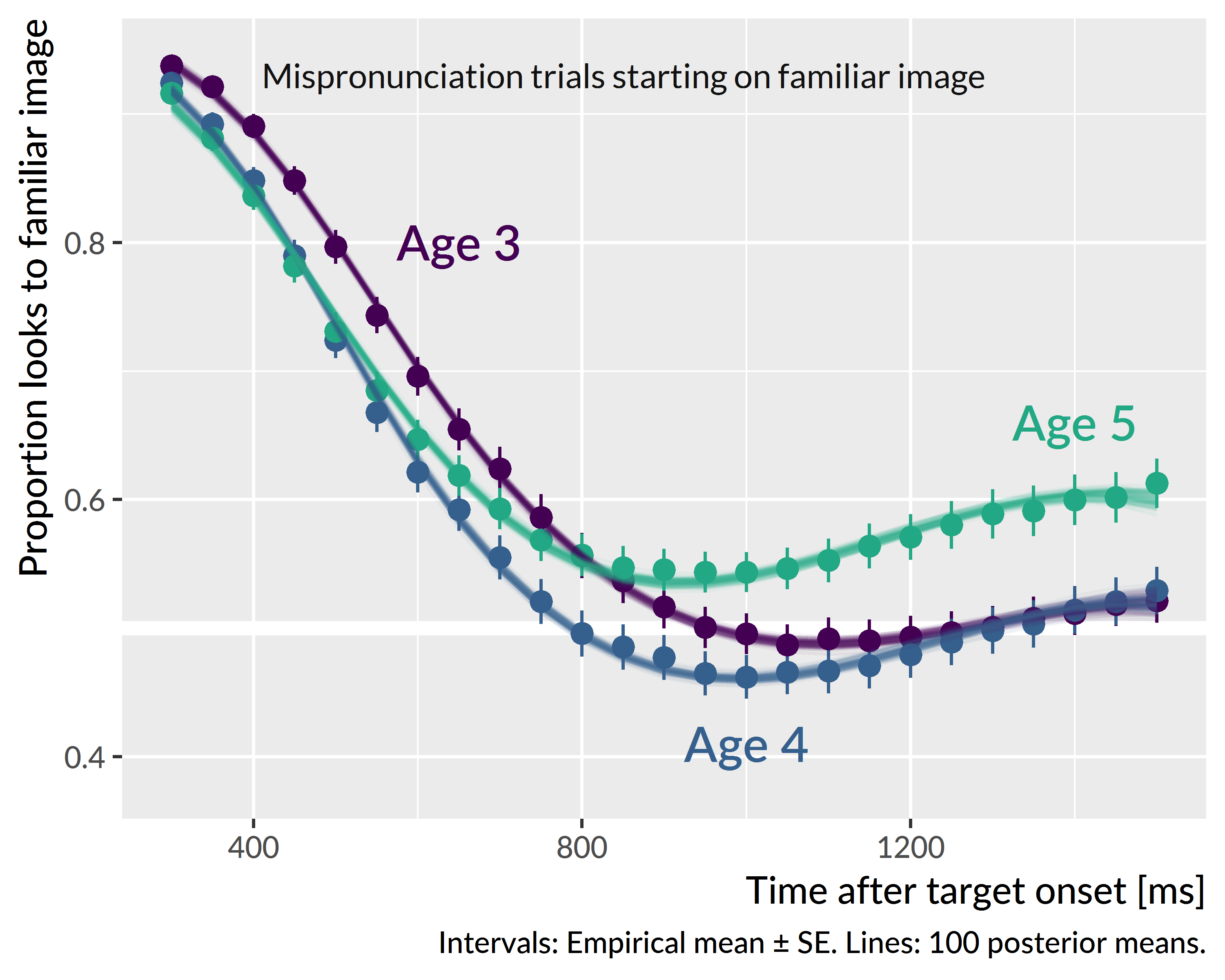
Figure 12.4: Average looks to familiar image for mispronunciation trials starting on the familiar image at each age. Lines represent 100 posterior predictions of the group average (the average of participants’ individual growth curves).
In other analyses, growth curves rise and plateau, and age-related effects appear in how quickly the curves rise or the height at which they plateau. In those cases, it is straightforward to interpret how the intercept and linear time effects contribute to the curve’s shape over development. For this model, the curves fall and plateau, and there is not an obvious developmental, year-over-year change among the curves. Thus, more effort is required to interpret the model parameters and how they combine to form the growth curve shape.
Figure 12.5 visualizes how the growth curve features are weighted at each year and how they contribute to the overall growth curve shape. At age 3, the intercept feature, or average proportion of looks to the familiar image, was .68 [90% UI: .65, .71]. The feature is less meaningful in this situation because the curves all start at a high probability which inflates the average value. That said, comparisons remain useful. At age 4, the average probability decreased by .05 [.02, .09] to .63 [.60, .66], and at age 5 the average probability returns to age-3 levels, .68 [.65, .71]. This intercept effect contributes to how the age-4 curve dips below the others and indeed briefly crosses the .5 probability threshold.
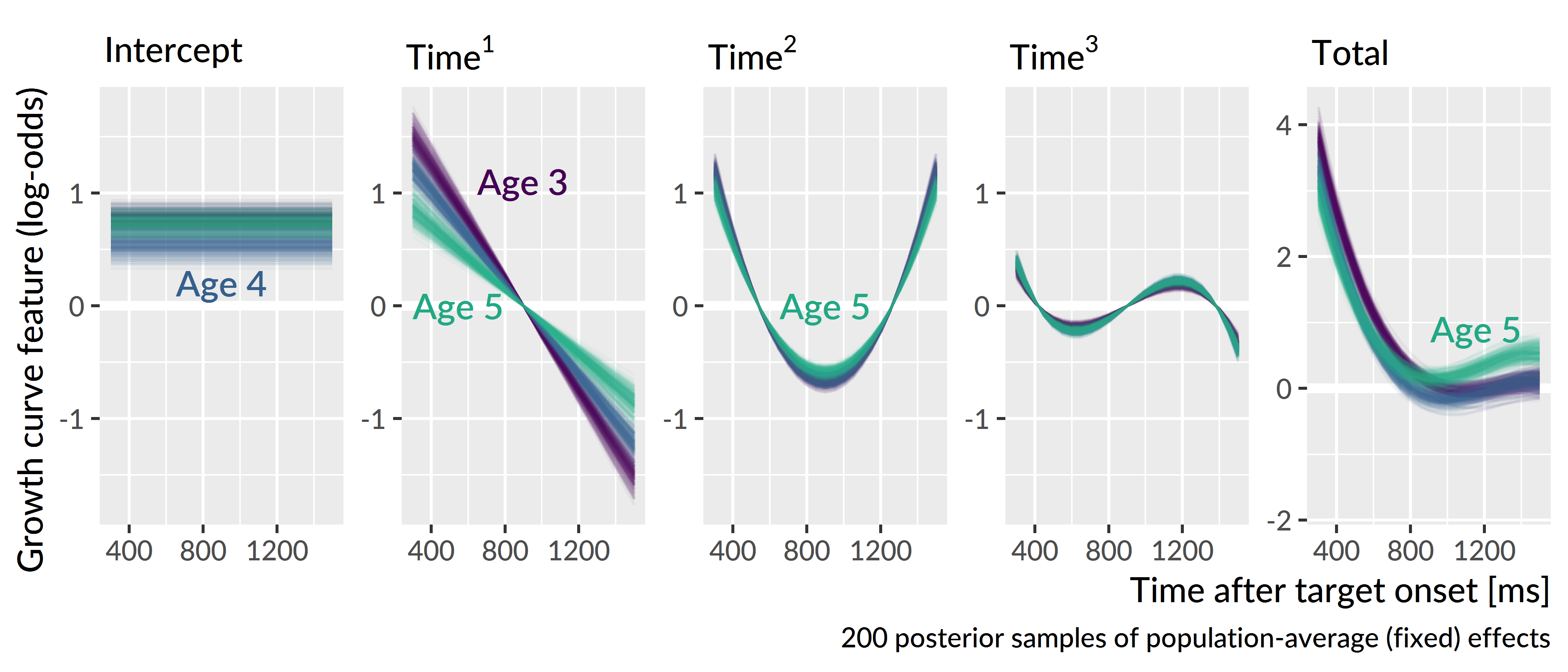
Figure 12.5: Weighted growth curve features. For the first four panels, the y axes are scaled to the same range. This scaling highlights how the cubic time component contributes less to the overall shape than the other features.
For the linear time feature, the slope becomes flatter year over year, decreasing by 19.0% [7.00%, 29.0%] from age 3 to age 4 and decreasing by 30.0% [17.0%, 42.0%] from age 4 to age 5. For these curves, however, the starting location is the highest value on the curve, so the linear time feature in this case mostly works to set the starting location of the curves. When the features are combined in Figure 12.5, the age-3 curve, which has the steepest linear time feature, starts at a higher value than the others.
There was a credible change in the quadratic time feature at age 5. One way to think of a positive quadratic trend is like a weight hanging on a string: It pulls and bends the whole curve downwards. At age 5, the quadratic feature is 12.0% [1.00%, 22.0%] smaller than at age 4, meaning that the age-5 curve has slightly less bend downwards. Finally, there were no credible differences in the cubic time feature. Compared to the other features, the cubic trend contributes only a small amount to the overall shape of the curves.
The combination of these effects shows in the final panel of Figure 12.5. The age-4 curve dips down furthest beneath 0 log-odds (.5 probability)—this is driven by in the intercept feature. The age-5 curve stays above 0 log-odds and eventually starts to rise away from its minimum value, owning to the dampened linear and quadratic features.
Summary. The shape of the average growth curves changed with each year of the study. Given the interplay of the curve features, I will avoid assigning a developmental interpretation to individual features. There are two main noticeable developmental trends at play however. First, the age-3 curve starts to fall from its baseline probability a little later than the other curves. Second, the age-5 curve stays above .5 probability and starts to rise at the end of the trial. At age 5, children were more likely to stay looking at the familiar object than look at both images equally.
12.2.1 Child-level predictors and different listening behaviors
In other word recognition analyses, I derived a growth curve “peak” value as a measure of maximum looking probability or minimum word recognition uncertainty. For these trials, I asked whether analogous growth curve “valleys” provided a meaningful feature for looking behavior when children start a trial fixated on the familiar image. This value was defined as the median of the five smallest values of a growth curve. Intuitively, it reflects the maximum degree to which the novel image is considered as a referent for the mispronunciation.
Figure 12.6 shows the posterior means of participants’ growth curve valleys. Note that there is considerable variability at each age, with the 0–1 interval nearly covered at age 4. The median value is closer to .5 at age 5, and this difference is consistent with the growth curve trajectories where the average age-5 curve did not dip as low as the other curves.
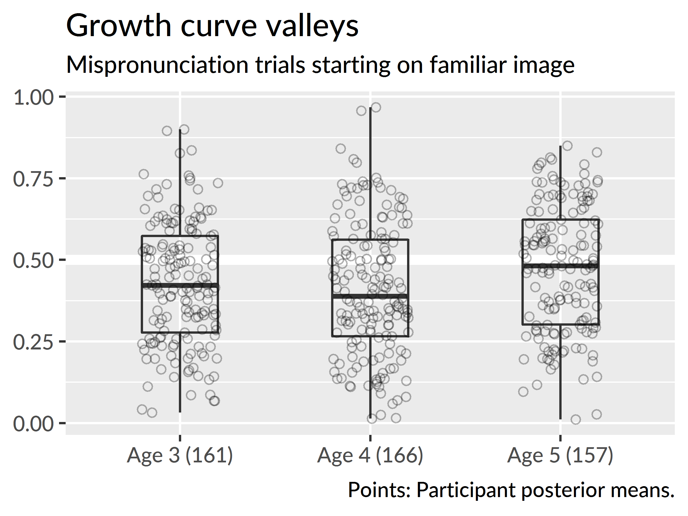
Figure 12.6: Growth curve valleys by age for mispronunciation trials starting on the familiar image.
The wide range of values for the growth curve valleys suggests that there are a few different listening behaviors that are being averaged over in the above analyses. The valleys above .6, for example, indicate that some children on average stay with the familiar image, and the valleys below .4 indicate children who favor the unfamiliar image.
To explore individual listening behaviors, I visualized children’s individual growth curves based on their growth curve valleys. Within each year, I grouped children into sextiles based on the posterior mean of their valleys and plotted their individual growth curves. Figure 12.7 shows the results from age 3. The final two bins show children who stayed with the familiar image throughout the mispronunciation trials. The first two bins mostly contain children who switched to the unfamiliar image and stayed there. These are also children whose curves show a pronounced u-shaped trajectory. Specifically, the curves with the highest ending points in the first three bins highlight children with u-shaped trajectories. In these curves, the probability of fixating on the familiar image briefly decreases, as the child considers the other image.
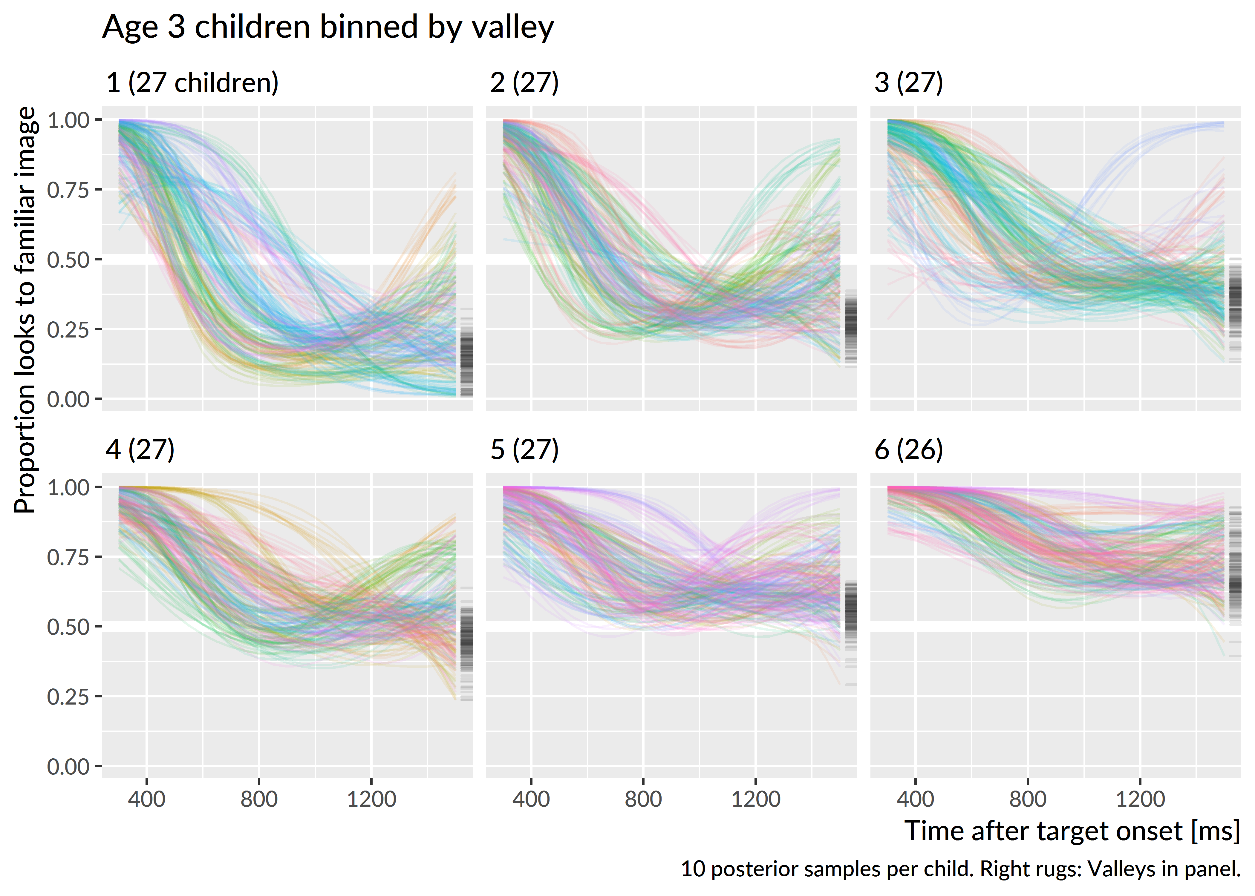
Figure 12.7: Growth curves for mispronunciation trials starting on the familiar image at age 3. Children were grouped into sextiles based on the posterior mean of their growth curve valleys—that is, the lowest point on the growth curve. Ten lines are drawn per child to visualize uncertainty. Children were assigned colors arbitrarily. On the right side of each panel are “rugs” which mark the valleys in that panel.
I asked whether any child-level factors predicted children’s looking behaviors. I first regressed growth curve valleys on EVT-2 standard score. There was a small effect at age 3, R2 = .09, n = 145. A 15-point increase in expressive vocabulary predicted decrease in growth curve valley of .05. At the other ages, the effects are negligibly small, as shown in Figure 12.8.
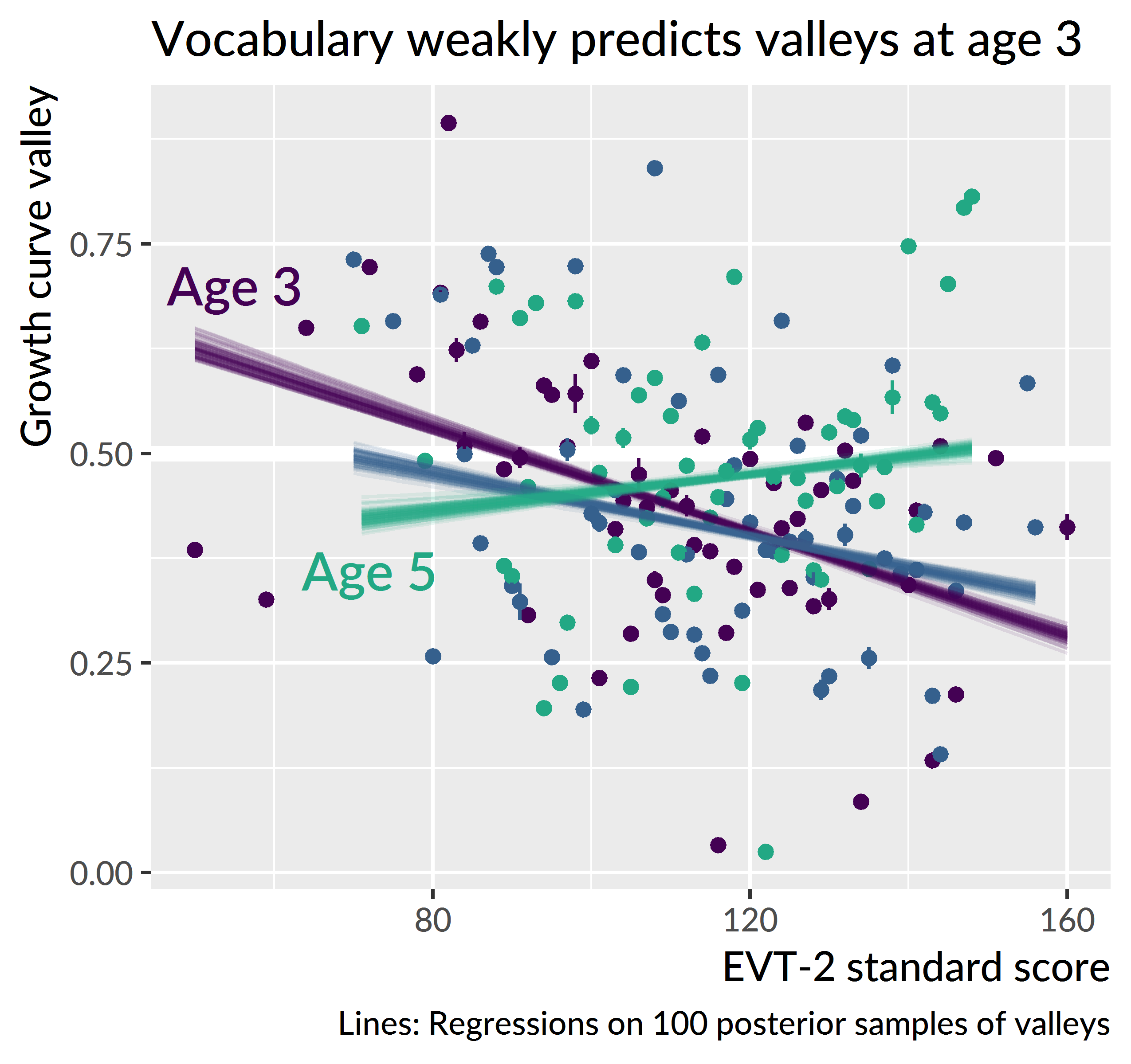
Figure 12.8: Relationship between expressive vocabulary and growth curve valleys for mispronunciation trials starting on the familiar image.
I regressed age-3 valleys onto expressive vocabulary, minimal-pair discrimination accuracy, and their interaction. The two main effects and their interaction were all statistically significant, R2 = .17, n = 139. The effects of vocabulary and minimal-pair discrimination were both negative, so that higher scores on these measures predicted lower growth curve valleys—that is, a greater maximum probability of fixating on the unfamiliar image. For an average participant, a 15-point increase in expressive vocabulary predicted a decrease of .03, and an increase of minimal pair accuracy of .1 predicted a decrease in valley of .03. The interaction term, however, was positive, meaning that increasing one of the predictors simultaneously weakens the effect of the other. As one of the predictors increases, it can push the effect of the other closer to zero so that its simple effect is “no longer” statistically significant. In this case, the simple effect of expressive vocabulary was not significant when minimal pair accuracy was .71 or greater (that is, at the 60-percentile or greater). Conversely, the simple effect of minimal pair discrimination accuracy was not significant when expressive vocabulary standard score was 119 or greater (at the 60-percentile or greater). In summary, at age 3, both expressive vocabulary and minimal pair discrimination each predicted greater consideration of the unfamiliar image. But these effects also interacted so that a large change in one predictor would weaken the effect of the other.
The growth curve valley feature measures the maximum extent to which the novel object is considered as the referent on these trials. But the u-shaped growth curves in Figure 12.7 suggest another listening response on this task: Confirmatory looks to the unfamiliar object. In these u-shaped curves, a child’s probability of fixating on the familiar object temporarily decreases as the novel object is considered, and the probability rises as that interpretation is rejected. To quantify this tendency, I computed each child’s growth curve on the probability scale and re-estimated the quadratic trends in these curves. Exploratory visualization showed that children with higher values on this quadratic trend were more likely to have a u-shape curve. This feature, however, also favored sigmoid or z-shaped curves that rapidly fell and plateaued. To avoid these kinds of curves, I weighted the quadratic trend using the median of the final five points of the curve. The weighted quadratic feature penalized curves that have a strong quadratic trend but end on a low probability. Figure 12.9 shows growth curves of age-5 children binned using this feature. The bottom row of panels illustrates how the u-shaped feature becomes stronger in each bin. The weighted quadratic feature was weakly correlated with the growth curve valleys, r = −.12, and the lack of correlation appears in the figure by how the curves in each panel reach different valleys.
Figure 12.9: Growth curves for mispronunciation trials starting on the familiar image at age 5. Children were grouped into sextiles based on the posterior mean of their curves quadratic trend weighted by the height of the curve in the final time bins. Ten lines are drawn per child to visualize uncertainty. Children were assigned colors arbitrarily.
I regressed the u-shaped curve feature onto expressive vocabulary standard score at each age and onto minimal pair discrimination for age 3. There was a tiny yet significant effect of vocabulary at age 5, R2 = .03, where children with lower vocabularies had a slightly stronger u-shaped trend in their growth curve. This effect, however, is so small as to be negligible. None of the effects were significant.
Summary. At age 3, children with larger expressive vocabularies or better minimal pair discrimination had lower growth curve valleys—that is, they looked more to the unfamiliar object when they heard a mispronunciation while fixated on an image of the mispronounced word. These two child-level measures significantly interacted so that increasing both measures simultaneously had diminishing returns. I devised a measure of the how u-shaped the growth curves were, but there were not any meaningful effects of vocabulary or expressive vocabulary on this measure.
12.3 Looking behaviors and word learning
At age 5, we tested children’s retention of the novel objects paired with the mispronunciations and nonwords. Children saw the two novel objects and heard either the mispronunciation or the nonword, and they had to point to the objects that went with the image. All six nonwords and mispronunciations were tested.
Table 12.1 shows the results for each item. Overall, children performed better on the nonwords than the real words. Children performed decidedly better on the nonwords than the mispronunciations on four of the pairs and performed about equally well on the remaining two (gake–pumm, wice–bape).
| Word Group | Type | Item | Trials Correct | Percent Correct ± SE |
|---|---|---|---|---|
| cake | mispronunciation | gake | 61 / 107 | 57.0% ± 4.8 |
| nonword | pumm | 56 / 107 | 52.0% ± 4.8 | |
| duck | mispronunciation | guck | 71 / 107 | 66.0% ± 4.6 |
| nonword | shann | 97 / 107 | 91.0% ± 2.8 | |
| girl | mispronunciation | dirl | 71 / 107 | 66.0% ± 4.6 |
| nonword | naydge | 98 / 107 | 92.0% ± 2.7 | |
| rice | mispronunciation | wice | 79 / 107 | 74.0% ± 4.2 |
| nonword | bape | 80 / 107 | 75.0% ± 4.2 | |
| shoes | mispronunciation | suze | 60 / 107 | 56.0% ± 4.8 |
| nonword | geeve | 90 / 107 | 84.0% ± 3.5 | |
| soup | mispronunciation | shoup | 63 / 107 | 59.0% ± 4.8 |
| nonword | cheem | 93 / 107 | 87.0% ± 3.3 | |
| (all) | mispronunciation | 405 / 642 | 63.0% ± 1.9 | |
| nonword | 514 / 642 | 80.0% ± 1.6 |
I performed an item-response analysis using a mixed-effects logistic regression model. Appendix D reports the code used to specify the model. The model included varying intercepts for child, child × item type, item, and word-group. The first two effects capture information about a child’s general ability and their ability on each type of item. The second two effects capture information about an item’s difficulty and difficulty of object-pairs. I also asked whether growth curve peaks predicted novel word recognition accuracy, so I included growth curve peaks from each condition in the model. For the nonwords, I used the age-5 peak proportion of looks to the novel image for trials that started on the familiar object. For the mispronunciations, I used the peak looks to the familiar object on trials that started on the unfamiliar object. I chose those peaks based on the conclusion that children were reliably treating the mispronunciations as imperfect productions of the familiar word. The model included data from 101 children.
The model confirmed that children were much more successful on the nonword trials. For a child with an average mispronunciation peak (.72), the predicted proportion correct on the mispronunciation retention trials was .64 [.49, .76]. A 1-SD (.19) increase in the mispronunciation peak predicted a change in proportion correct of −.05 [−.10, −.01]. Children who looked more to the familiar object on these mispronunciation trials were less successful during the retention trials. For a child with an average peak on the nonword trials (.90), the predicted proportion correct on the nonword retention trials was .82 [90% UI: .70, .89]. A 1-SD increase (.10 to 1.00) in nonword peaks predicted a change in proportion correct of −.01 [−.05, .02]. The uncertainty interval here includes positive and negative values. It is uncertain whether the effect is positive or negative, so I conclude that there was not a reliable effect in the nonword case.
Figure 12.10 visualizes the model results. The difference in height between the two curves reflects the general advantage in the nonword condition. The negative slope for the mispronunciation line captures the effect of growth curve peaks. A change in mispronunciation growth curve peak from .5 to 1 roughly predicts a change from 4/6 to 3/6 mispronunciation items correct. The nonword line hovers around 5/6 items correct: There is not enough information in the peaks or in the number of retention trials for a reliable effect to emerge.
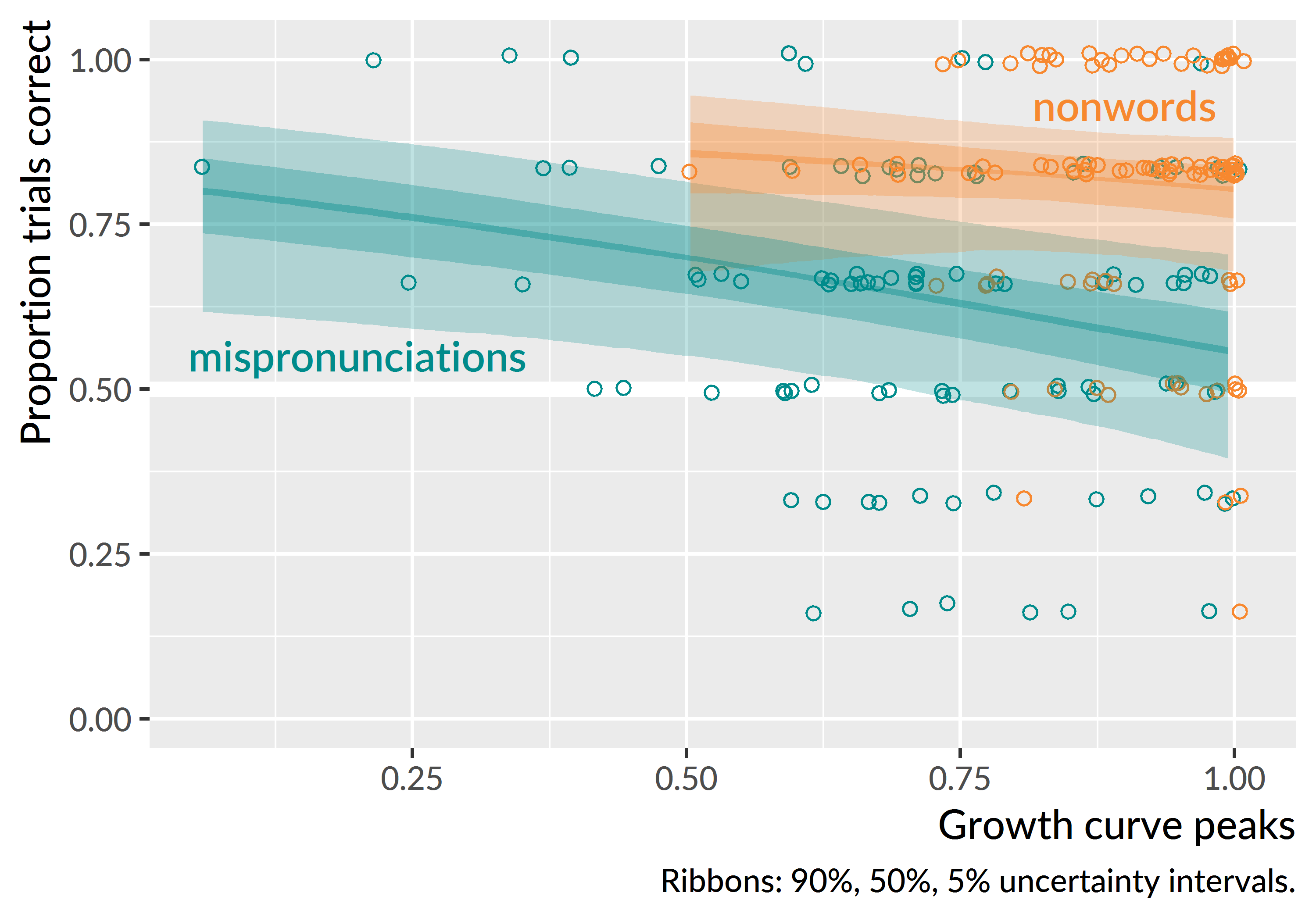
Figure 12.10: Effect of growth curve peaks on children’s accuracy on retention trials. For the mispronunciations, I used the peak looks to the familiar image on trials where the child started on the unfamiliar image, so it represents, say, how much a child looked at shoes given “suze”. Thus, more permissive listeners looked performed more poorly on the retention trials. For the nonwords, I used the peak look to the unfamiliar image on trials where the child started on the familiar image. Points were jittered by 1% to avoid overplotting. There were six trials per condition which is why the points fall into 6 bands.
Summary. When 5-year-olds were tested on their retention of the unfamiliar images used on the mispronunciation and nonword trials, children were much more accurate for the nonwords than the mispronunciations. Children’s accuracy on the mispronunciations was related to their looking behaviors: Children who looked more to the familiar image during mispronunciation trials had a lower accuracy on the mispronunciation retention trials.
12.4 Discussion
In the lab, when preschoolers are looking at a novel object and hear the name of a different familiar object, albeit mispronounced, they look to the familiar object. Children do this reliably at age 3 and even more reliably at age 5. Thus, children recognized these mispronunciations as productions of familiar words, but this recognition was not without a penalty. They looked much less to the familiar object under these conditions, compared to trials where they hear a correct production of the familiar object—see Figure 12.11—or when they hear a nonword in a context that supports fast-referent selection. Therefore, preschoolers are unquestionably sensitive to mispronunciations of familiar words, as they show more uncertainty when hearing a mispronunciation.
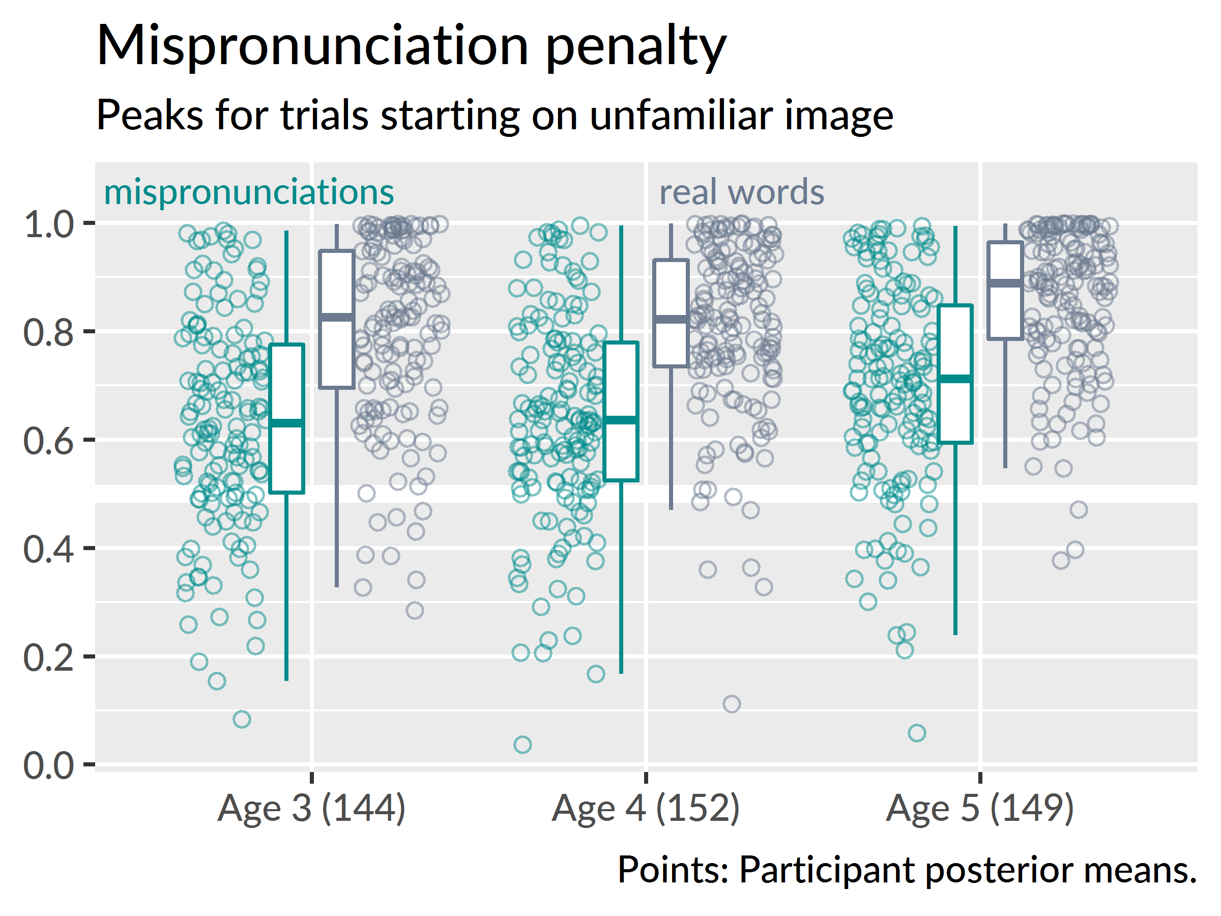
Figure 12.11: Comparison of growth curve peaks for the real words and mispronunciations.
Child-level measures generally did not predict how well children tolerated mispronunciations. There was a very small effect of expressive vocabulary at age 3 such that children with larger vocabularies looked more the familiar image on these trials. Although children differed in their tendency to look to a familiar image when given a mispronunciation, these differences could not be pinned to any child-level measures.
I also analyzed trials where children started on the familiar word and heard a mispronunciation. In this situation, there is no one clear strategy for referent selection, and children exhibit a few different patterns. Some listeners stay with the familiar image. Some reliably switch to the novel image. Some look at both equally. On average, the growth curve averages rush to .5—equal looking to both images and maximum uncertainty. At age 5, the curve does not reach quite as far down as the other curves, so they never demonstrate this degree of uncertainty. These sets of analyses mainly demonstrate that when children start on a familiar image and hear a mispronunciation, they have a few options for how to proceed.
Child-level predictors only were predictive at age 3 for curve valley. In this case, children with larger vocabularies or better minimal pair discrimination showed more consideration of the nonword object. I speculate that in this situation, the effect reflects that children with better abilities in these areas were more sensitive to the mispronunciation. These children were better at recognizing the mismatch from partial information and thus allocated more credibility to the alternative image.
One strategy to resolve the uncertainty in this situation would be to verify and reject the other image. Therefore, I also defined a weighted quadratic growth curve feature that measured how u-shaped the curves were. Such curves would reflect a child temporarily decreasing looks to the familiar image as a confirmatory looking behavior. The u-shaped curve features were not reliably related to any child-level factors, outside of negligibly small effect of expressive vocabulary at age 5.
Children demonstrated different looking behaviors based on their initial fixation location. For unfamiliar-initial trials, the growth curves show a reliable shift to the familiar image and we infer that the children treat the mispronunciation as passable production of the familiar word. For the familiar-initial trials, the children show much more uncertainty and a reliable advantage for the familiar word only begins to appear by age 5.
What are children doing in this situation? I initially thought that some children might “be finished” with the trial when they hear the word. That is, the child fixates on the familiar word, hears the mispronunciation prompt, notices that they have already found the image, and then looks to other parts of the screen. The problem with this possibility is that it does not happen in other conditions. For the nonword and real word conditions, when children start on the named image, they stick with the target. The average empirical growth curves in Figure 10.4 and Figure 10.5 tend to stay around 70–80% looking to the target image. Rather than reflecting disengagement from the task, the looking patterns indicate increased uncertainty in these trials.
Another possibility is that children show increased uncertainty because the mispronunciation effect is greater when the child is fixating on the familiar word. That is, children who fixated on the familiar image might have internally named the object and built up the word’s resting activation. The mispronunciation directly conflicts with the child’s pre-naming expectations for the word’s name, thus inducing more uncertainty after the word is named. For the unfamiliar-initial trials, on the other hand, a child’s attention is on the novel object and they have a less potent expectation about the words they might hear.
Visual attention did seem to influence how children retained information from the mispronunciation trials. At age 5, we tested children’s retention of the mispronunciations and nonwords. Children were much more likely to recall which unfamiliar object appeared on the nonword trials than the mispronunciation trials. This difference is not unexpected. In the nonword trials, children looked to an unfamiliar object when given an unambiguous novel word for a label. Thus, each trial worked to build an association between a new word and an unfamiliar object. But children generally treated the mispronunciations as productions of the familiar words. For the unfamiliar-initial trials, they looked more to the familiar object, a result that held at all three ages. Rather than developing a new object-label mapping, children are working on resolving an ambiguous and uncertain production on these trials. This idea is consistent with the effect of growth curve peaks on retention accuracy: Children who looked less to the unfamiliar object on mispronunciation trials were less likely to recall that unfamiliar object during retention testing.