Chapter 5 Analysis of familiar word recognition
5.1 Growth curve analysis
The outcome measure of interest here is how the probability of fixating on the target image versus the distractors changes over time. There are many possible techniques one can employ for modeling time series data. In this chapter, I used growth curve analysis which uses polynomial functions of time (a linear trend, a quadratic trend, etc.) to estimate a time series. Barr (2008) and Mirman, Dixon, and Magnuson (2008) are important early tutorials for this technique of modeling looking probabilities. (Incidentally, the two articles were published together in a special issue of Journal of Memory and Language about “emerging” statistical techniques.) Mirman (2014) also provides a textbook treatment of growth curve analysis for eyetracking data. This approach is well suited for time series where the trajectory is relatively simple with one or two inflection points. Alternatively, one can forgo polynomial trends and use generalized additive (mixed) models to fit a more general nonlinear shape. I apply this now-emerging technique in Chapter 6 to model wigglier growth curve shapes. A third possibility is to use nonlinear, functional growth curves. For the polynomial and additive models, underlying time features are weighted and summed to fit a nonlinear shape. For the functional growth curve, the nonlinear shape is fixed in advance and the model estimates a set of curve parameters so the shape approximates the data. For example, Oleson, Cavanaugh, McMurray, and Brown (2017) and Seedorff, Oleson, and McMurray (2018) model eyetracking data by assuming an s-shaped curve (a logistic function) and then estimating the left and right asymptotes, the slope at the steepest point, and the point where the steepest rise occurs. These parameters are directly interpretable in terms of looking behaviors, but I have found that the technique is not flexible enough to handle the noisier shapes of children’s eyetracking data.3 For the following analyses, therefore, I used polynomial growth curves.
Looks to the familiar image were analyzed using Bayesian, mixed effects logistic regression. I used logistic regression because the outcome measurement is a probability (the log-odds of looking to the target image versus the distractors). I used mixed-effects models to estimate a separate growth curve for each child (to measure individual differences in word recognition) but also treat each child’s individual growth curve as a draw from a distribution of related curves. I used Bayesian techniques to study a generative model of the data. Instead of reporting and describing a single, best fit of some data, Bayesian methods consider an entire distribution of plausible fits that are consistent with the data and any prior information we have about the model parameters. By using this approach, one can explicitly quantify uncertainty about statistical effects and draw inferences using estimates of uncertainty (instead of using statistical significance—which is not a straightforward matter for mixed-effects models).4
Word recognition growth curves—that is, looks to the target versus the distractors at 250 ms, 300 ms, etc.—were fit using an orthogonal cubic polynomial function of time. Put differently, I modeled the probability of looking to the target during an eyetracking task as:
\[ \text{log\,odds}(\text{looking}) = \beta_0 + \beta_1\text{Time}^1 + \beta_2\text{Time}^2 + \beta_3\text{Time}^3 \]
That the time terms are orthogonal means that \(\text{Time}^1\), \(\text{Time}^2\) and \(\text{Time}^3\) are transformed so that they are uncorrelated. See Box 1. Under this formulation, the parameters \(\beta_0\) and \(\beta_1\) have a direct interpretation in terms of lexical processing performance. The intercept, \(\beta_0\), measures the area under the growth curve—or the probability of fixating on the target word averaged over the whole window. We can think of \(\beta_0\) as a measure of word recognition reliability. The linear time parameter, \(\beta_1\), estimates the steepness of the growth curve—or how the probability of fixating changes from frame to frame. We can think of \(\beta_1\) as a measure of processing efficiency, because growth curves with stronger linear features exhibit steeper frame-by-frame increases in looking probability.
Box 1: Orthogonal time.
I used orthogonal polynomial features of Time for these growth curve models. Unlike natural polynomials, these features are uncorrelated. This aspect makes these models more flexible: I do not have to worry about any collinearity between Time1 and Time2. Moreover, adding an orthogonal cubic Time3 term to a quadratic model will not change any of the estimates for Time1 or Time2 because the added predictor is not correlated with the others. One disadvantage of this approach is that the features are not as straightforward to interpret.
The figure below shows the orthogonal polynomials used by the model and how they can be weighted and summed to fit a growth curve.
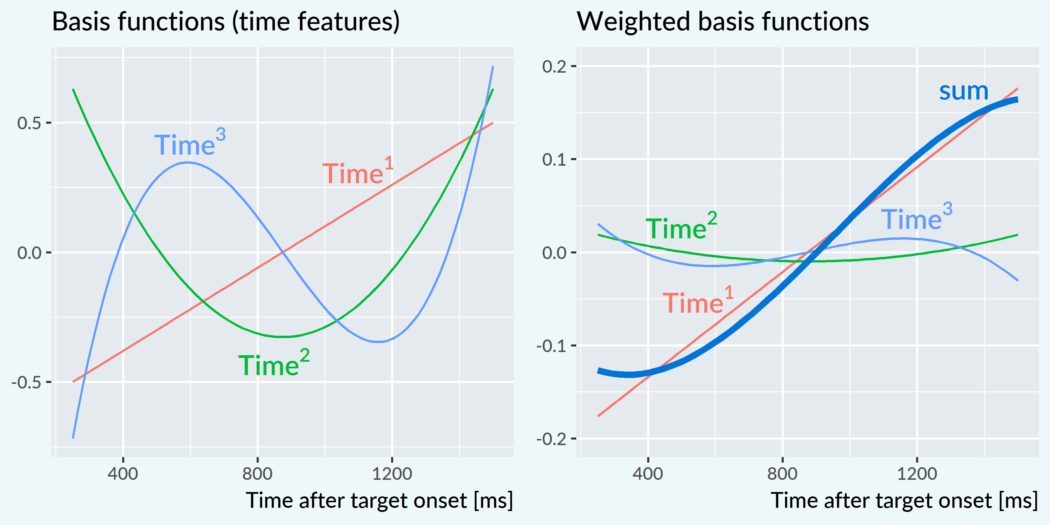
Note that the time features and weighted features are vertically centered around 0. The curves are adjusted up or down to their correct position by the model’s intercept term. Conceptually, one can also think of the intercept as a Time0 feature—that is, a horizontal line at y = 1 which is weighted to move the whole curve vertically. This is why in these models, the intercept is not the value at some time 0 but rather the average value of the fitted growth curve. To reiterate, for these word recognition models, the intercept is the average probability of the curve.
For all the polynomial growth curves models I used in this project, I scaled the features so that Time1 ranges from −.5 to .5. In other words, a 1-unit change on Time1 marks the whole traversal across the analysis window. After scaling, Time2 ranges from −.33 to .60 and Time3 ranges from −.63 to .63.
In my experience, only the intercept terms and linear time trends of an orthogonal polynomial model have a behaviorally straightforward interpretation. The polynomial other terms are less important—or rather, they do not map as neatly onto behavioral descriptions as the accuracy and efficiency parameters. The primary purpose of quadratic and cubic terms is to ensure that the estimated growth curve adequately fits the data. In this kind of data, there is a steady baseline at chance probability before the child hears the word, followed a window of increasing probability of fixating on the target as the child recognizes the word, followed by a period of plateauing and then diminishing looks to target. The cubic polynomial allows the growth curve to be fit with two inflection points: the point when the looks to target start to increase from baseline and the point when the looks to target stops increasing.
To study how word recognition changes over time, I modeled how the growth curves change over developmental time. This amounted to studying how the growth curve parameters changes year over year. I included dummy-coded indicators for age 3, age 4, and age 5 and allowed these indicators to interact with the growth curve parameters:
\[ \small \begin{align*} \text{log\,odds}(\text{looking}) =\ &\beta_0 + \beta_1\text{Time}^1 + \beta_2\text{Time}^2 + \beta_3\text{Time}^3\ + &\text{[age 3 growth curve]} \\ (&\gamma_{0} + \gamma_{1}\text{Time}^1 + \gamma_{2}\text{Time}^2 + \gamma_{3}\text{Time}^3)*\text{Age\,4}\ + \ &\text{[age 4 adjustments]} \\ (&\delta_{0} + \delta_{1}\text{Time}^1 + \delta_{2}\text{Time}^2 + \delta_{3}\text{Time}^3)*\text{Age\,5} \ &\text{[age 5 adjustments]} \\ \end{align*} \normalsize \]
These year-by-growth-curve-feature terms captured how the shape of the growth curves changed each year. The model also included random effects to represent by-child and by-child-by-year effects to estimate a general growth curve for each child and to estimate how each child’s growth curve changed each year.
The models were fit in R (vers. 3.4.3) with the RStanARM package (vers. 2.16.3). Appendix B contains the R code used to fit the model along with a description of the model specifications represented in the model syntax.
I used Bayesian uncertainty intervals to draw statistical inferences. A Bayesian model is the posterior distribution: It is a distribution of plausible parameter values, given the data, a data-generating model and any prior information we have about those parameter values. In practice, these distributions are hard to calculate, so we use Markov Chain Monte Carlo to get a sample of thousands of values from the posterior distribution. Thus, rather than having a single best-fitting estimate of some effect \(\beta\), we have a sample of, say, 4,000 plausible values for \(\beta\). We can quantify our uncertainty about \(\beta\) by describing the distribution of those values. I use typically two statistics to describe that distribution. The median provides a point estimate for the distribution, and the 90% uncertainty interval provides bounds for the effect. These intervals have an intuitive interpretation. Suppose that for \(\beta\) we get a median of 8 and 90% uncertainty interval of [5, 21]. This interval means that we can be 90% certain that the “true” value of \(\beta\) is between 5 and 21, given the data, our model, and our prior information. Moreover, by inspecting the interval, we pinpoint areas of uncertainty. In this example, we can conclude that the effect is likely to be positive. The lower interval value of 5 tells us that 90% of the plausible values are greater than 5. A wide range of values are covered by the interval, however, so we would also conclude that we are not very certain about the size of the effect. It bears noting that one cannot interpret frequentist confidence intervals in this way. See Kruschke and Liddell (2017) for a recent review of frequentist versus Bayesian statistics.
5.1.1 Growth curve features as measures of word recognition performance
As mentioned above, two of the model’s growth curve features have straightforward interpretations in terms of lexical processing performance: The model’s intercept parameter corresponds to the average proportion or probability of looking to the named image over the trial window, and the linear time parameter corresponds to slope of the growth curve or lexical processing efficiency. I also was interested in peak proportion of looks to the target. I derived this value by computing the growth curves from the model and taking the median of the five highest points on the curve. Figure 5.1 shows three simulated growth curves and how each of these growth curve features relate to word recognition performance.
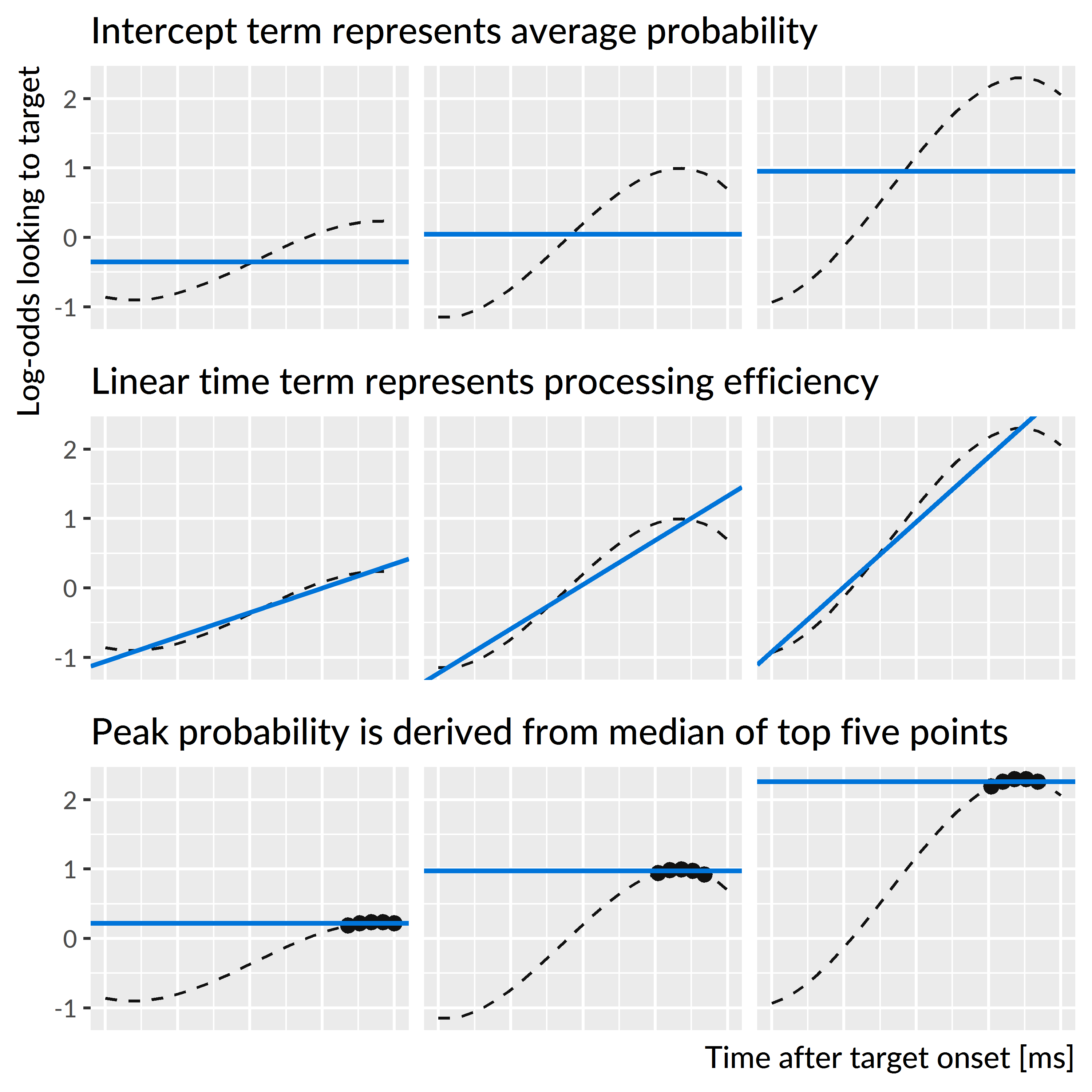
Figure 5.1: Illustration of the three growth curve features and how they describe lexical processing performance. The three curves used are simulations of new participants at age 4.
5.2 Year over year changes in word recognition performance
The mixed-effects model estimated a population-average growth curve (“fixed” effects) and how individual children deviated from the average (“random” effects). Figure 5.2 shows 200 posterior samples of the population-average growth curves for each year. On average, the growth curves become steeper and achieve higher looking probabilities with each year of the study.
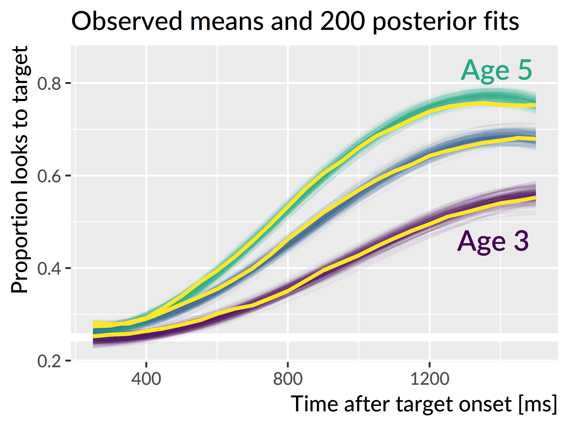
Figure 5.2: Population-average (“fixed effects”) word recognition growth curves at each age. Colored lines represent 200 posterior samples of these growth curves; these are included to visualize the uncertainty about the population averages. The thick light lines represent the observed average growth curve at each age.
Figure 5.3 depicts uncertainty intervals with the model’s average effects of each timepoint on the growth curve features. The intercept and linear time effects increased each year, confirming that children become more reliable and faster at recognizing words as they grow older. The peak probability also increased each year. For each effect, the change from age 3 to age 4 is approximately the same as the change from age 4 to age 5, as illustrated in Figure 5.4.
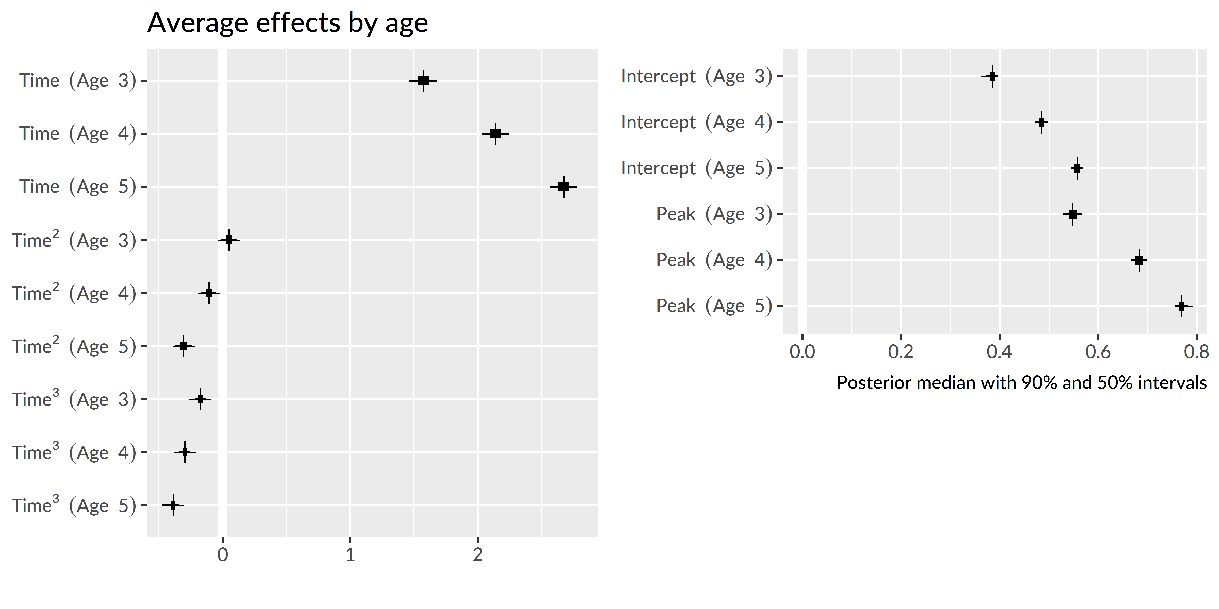
Figure 5.3: Uncertainty intervals for growth curve features at each age. The intercept and peak features were converted from log-odds to proportions to ease interpretation.
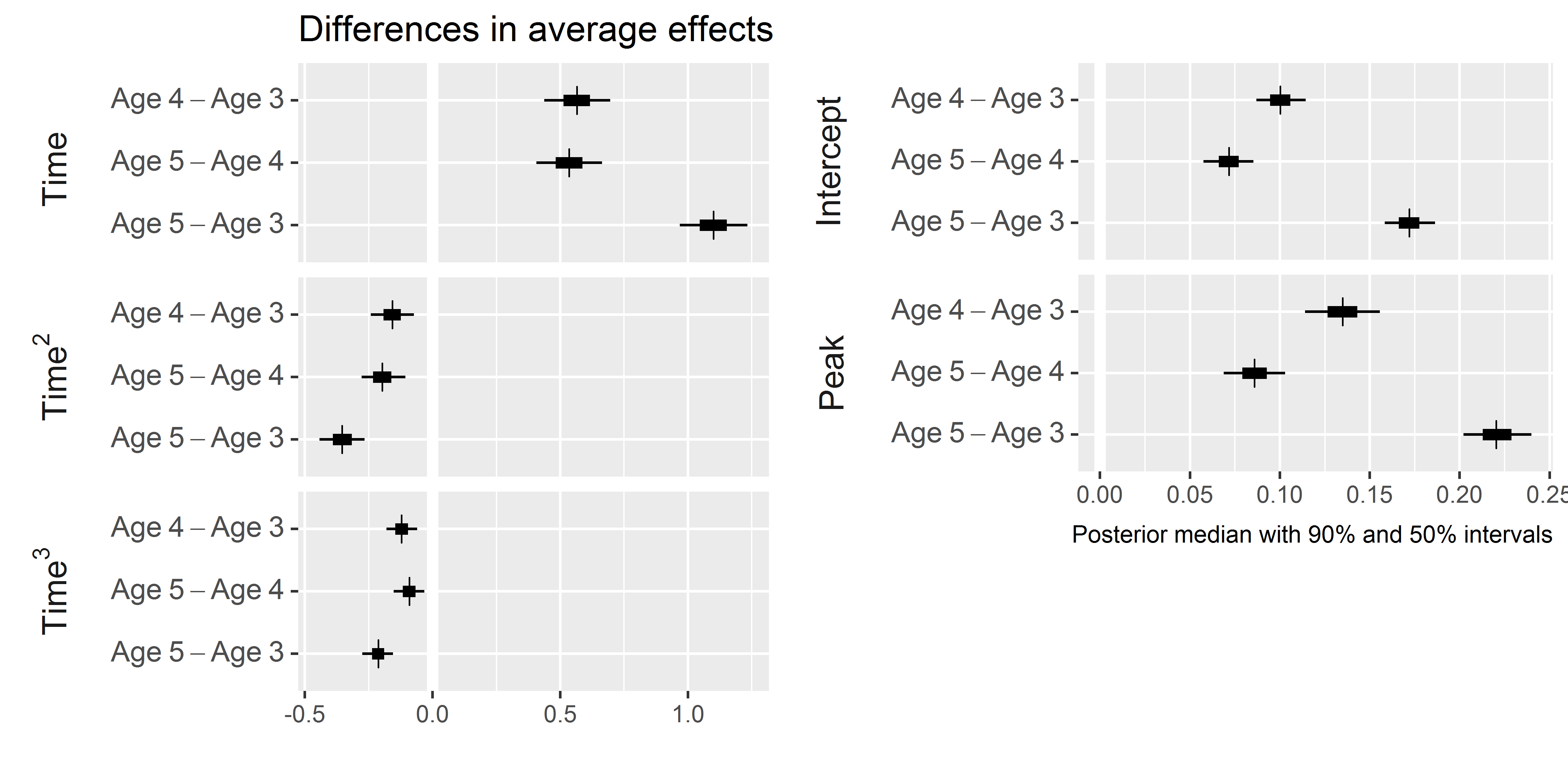
Figure 5.4: Uncertainty intervals for the differences in growth curve features between ages. Again, the intercept and peak features were converted to proportions.
The average looking probability (intercept feature) was 0.38 [90% UI: 0.37, 0.40] at age 3, 0.49 [0.47, 0.50] at age 4, and 0.56 [0.54, 0.57] at age 5. The averages increased by 0.10 [0.09, 0.11] from age 3 to age 4 and by 0.07 [0.06, 0.09] from age 4 to age 5. The peak looking probability was 0.55 [0.53, 0.57] at age 3, 0.68 [0.67, 0.70] at age 4, and 0.77 [0.76, 0.78] at age 5. The peak values increased by 0.13 [0.11, 0.16] from age 3 to age 4 and by 0.09 [0.07, 0.10] from age 4 to age 5. These results numerically confirm the hypothesis that children would improve in their word recognition reliability, both in terms of average looking and in terms of peak looking, each year. The changes in peak probability were also rather large: children’s probability fixating on the target increased by approximately .1 each year. These growths indicate the task scaled with children’s development because they had room to improve each year.
Summary. The average growth curve features increased year over year, so that children looked to the target more quickly and more reliably as they grew older.
5.3 Exploring plausible ranges of performance over time
Bayesian models are generative; they describe how the data could have been generated. This model assumed that each child’s growth curve was drawn from a population of related growth curves, and it tried to infer the parameters over that distribution. These two aspects—a generative model and learning about the population of growth curves—allow the model to simulate new samples from that distribution of growth curves. That is, we can predict a set of growth curves for a hypothetical, unobserved child drawn from the same distribution as the 195 children observed in this study. This procedure of studying model implications by having the model generate new data is called posterior predictive inference, and in this case, it allows one to explore the plausible degrees of variability in performance at each age.
Figure 5.5 shows the posterior predictions for 1,000 simulated participants, and it demonstrates how the model expects new participants to improve longitudinally but also exhibit stable individual features over time. Figure 5.6 shows uncertainty intervals for these simulations. The model learned to predict less accurate and more variable performance at age 3 with improving accuracy and narrowing variability at age 4 and age 5.
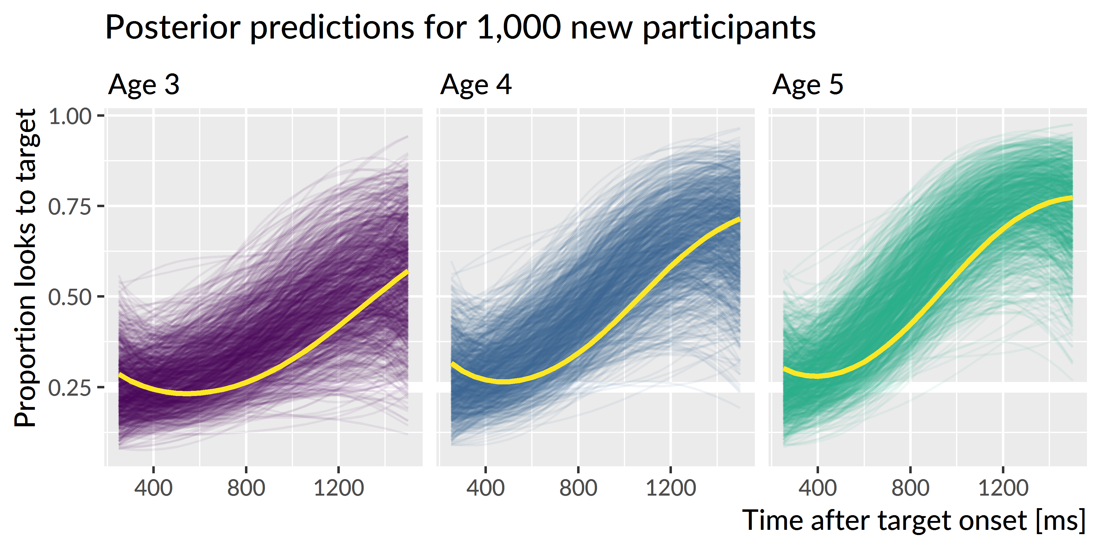
Figure 5.5: Posterior predictions for hypothetical unobserved participants. Each line represents the predicted performance for a new participant. The three light lines highlight predictions from one single simulated participant. The simulated participant shows both longitudinal improvement in word recognition and similar relative performance compared to other simulations each year, indicating that the model would predict new children to improve year over year and show stable individual differences over time.
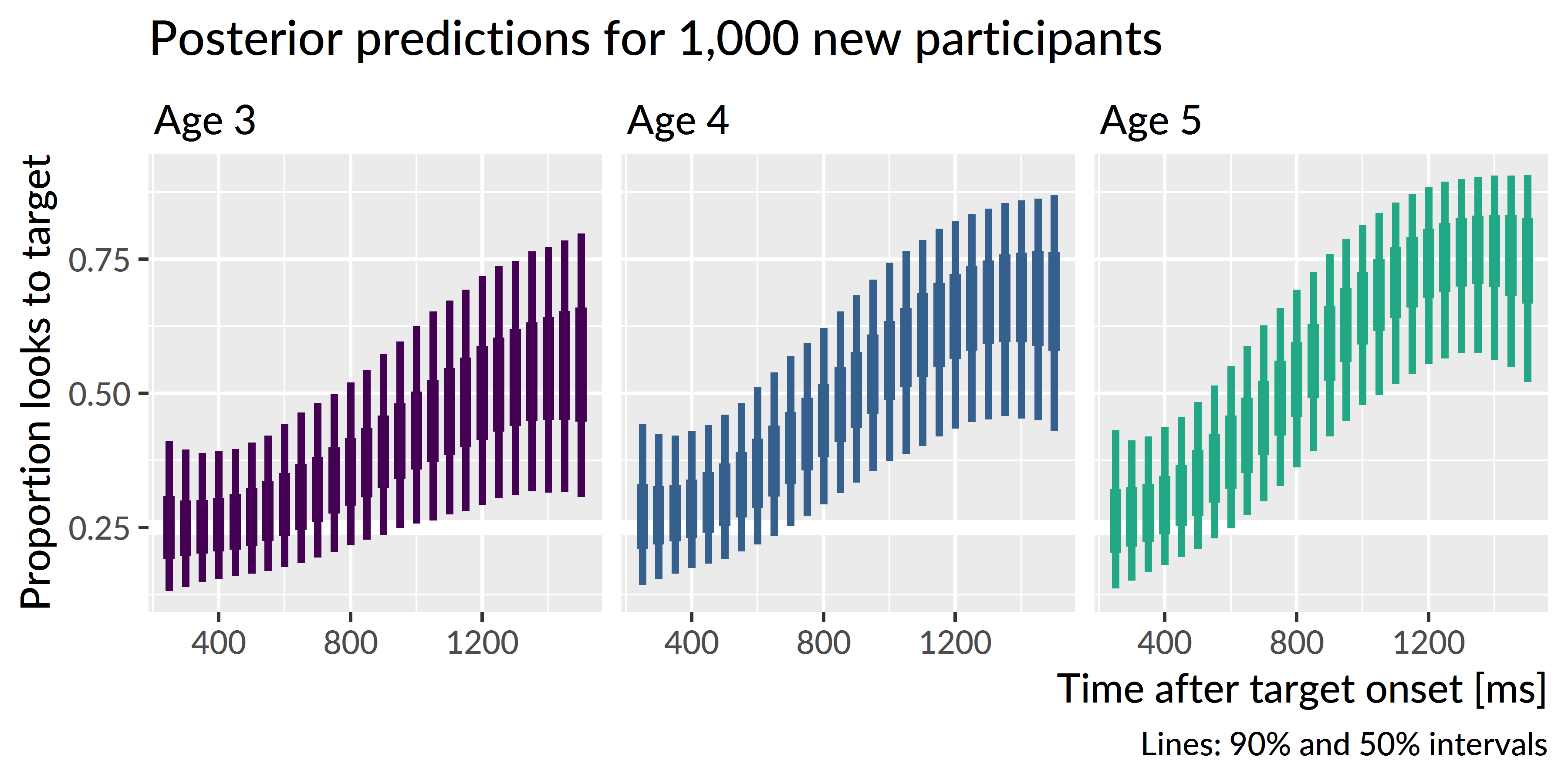
Figure 5.6: Uncertainty intervals for the simulated participants. Variability is widest at age 3 and narrowest at age 5, consistent with the prediction that children become less variable as they grow older.
I hypothesized that children would become less variable as they grew older and converged on a mature level of performance. To address this question, I inspected the ranges of predictions for the simulated participants. The claim that children become less variable would imply that the range of predictions should be narrower for age 5 than for age 4 and narrower for age 4 than for age 3. Figure 5.7 depicts the range of the predictions, both in terms of the 90-percentile range (i.e., the range of the middle 90% of the data) and in terms of the 50-percentile (interquartile) range. The ranges of performance decrease from age 3 to age 4 to age 5, consistent with the hypothesized reduction in variability.
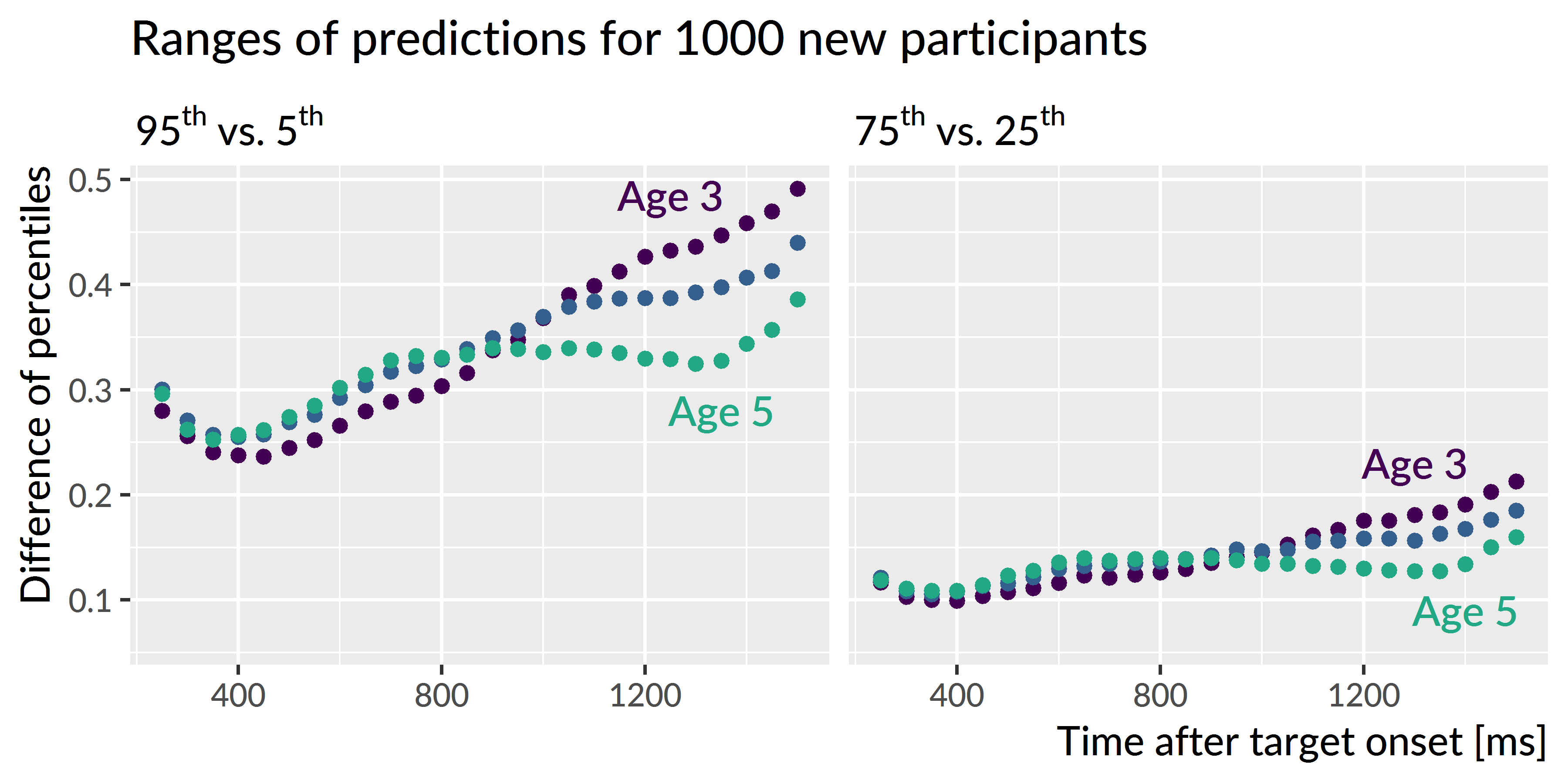
Figure 5.7: Ranges of predictions for simulated participants over the course of a trial. The ranges are most similar during the first half of the trial when participants are at chance performance, and the ranges are most different at the end of the trial as children reliably fixate on the target image. The ranges of performance decrease with each year of the study as children show less variability.
The developmental pattern of increasing reliability and decreasing variability was also observed for the growth curve peaks. For the synthetic participants, the model predicted that individual peak probabilities will increase each year, peak3 = 0.55 [90% UI: 0.35, 0.77], peak4 = 0.69 [0.48, 0.86], peak5 = 0.78 [0.59, 0.91]. Moreover, the range of plausible values for the individual peaks narrowed each for the simulated data. For instance, the difference between the 95th and 5th percentiles was 0.43 for age 3, 0.38 for age 4, and 0.32 for age 5.
Summary. I used the model’s random effects estimates to simulate growth curves from 1,000 hypothetical, unobserved participants. The simulated dataset showed increasing looking probability and decreasing variability with each year of the study. These simulations confirmed the hypothesis that variability would diminish as children began to demonstrate a mature degree of performance for this task.
5.4 Are individual differences stable over time?
I predicted that children would show stable individual differences such that children who are faster and more reliable at recognizing words at age 3 remain relatively faster and more reliable at age 5. To evaluate this hypothesis, I used Kendall’s W (the coefficient of correspondence or concordance). This nonparametric statistic measures the degree of agreement among J judges who are rating I items. For these purposes, the items are the 123 children who provided reliable eyetracking for all three years of the study. (That is, I excluded children who only had reliable eyetracking data for one or two years.) The judges are the sets of growth curve parameters from each year of study. For example, the intercept term provides three sets of ratings: The participants’ intercept terms from age 3 are one set of ratings and the terms from ages 4 and 5 provide two more sets of ratings. These three ratings are the “judges” used to compute the intercept’s W. Thus, I computed five groups of W coefficients, one for each set of growth curve features: Time1, Time2, Time3, average looking probability, and peak looking probability.
Because I used a Bayesian model, there is a distribution of ratings and thus a distribution of concordance statistics. Each sample of the posterior distribution fits a growth curve for each child in each year, so each posterior sample provides a set of ratings for concordance coefficients. This distribution of W’s lets us quantify our uncertainty because we can compute W’s for each of the 4000 samples from the posterior distribution.
One final matter is how to assess whether a concordance statistic is meaningful. To tackle this question, I also included a “null rater”, a fake parameter that assigned each child in each year a random number. I use the distribution of W’s generated by randomly rating children as a benchmark for assessing whether the other concordance statistics differ meaningfully from chance.
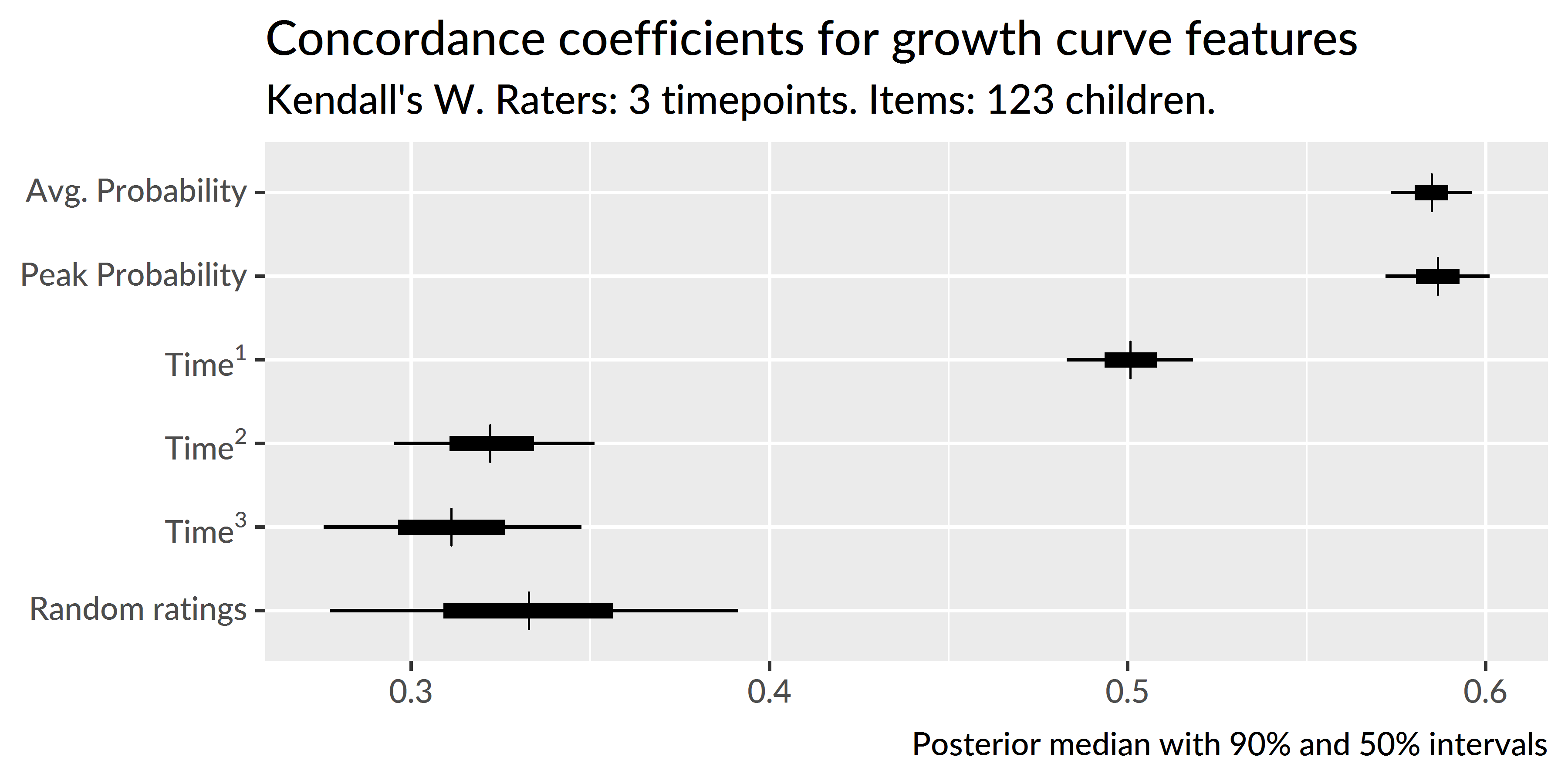
Figure 5.8: Uncertainty intervals for the Kendall’s coefficient of concordance. Random ratings provide a baseline of null W statistics. The peak, intercept and linear time features are decisively non-null, indicating a significant degree of correspondence in children’s relative word recognition reliability and efficiency over the three years of the study.
I used the kendall() function in the irr R package (vers. 0.84; Gamer, Lemon, & Singh, 2012) to compute concordance statistics. Figure 5.8 depicts uncertainty intervals for the Kendall W’s for these growth curve features. The 90% uncertainty interval of W statistics from random ratings, [.28, .39], subsumes the intervals for the Time2 effect [.30, .35] and the Time3 effect [.28, .35], indicating that these values do not differentiate children in a longitudinally stable way. Earlier, I claimed that only the intercept, linear time, and peak features have psychologically meaningful interpretations and that the higher-order time features mainly act to capture the curvature of the data. These null concordance statistics support that claim because the Time2 and Time3 features differentiate children across years as well as random numbers.
Concordance is strongest for the peak feature, W = .59 [.57, .60] and the intercept term, W = .58 [.57, .60], followed by the linear time term, W = .50 [.48, .52]. Because these values are far removed from the statistics for random ratings, I conclude that there is a credible degree of correspondence across years when ranking children using their peak looking probability, average look probability (the intercept) or their growth curve slope (linear time).
Summary. Growth curve features measured individual differences in word recognition performance. By using Kendall’s W to measure the degree of concordance among growth curve features over time, I tested whether individual differences in lexical processing persisted over development. I found that the peak looking probability, average looking probability and linear time features were stable over time. Children who were relatively fast (or reliable) at word recognition at one age were also relatively fast (or reliable) at other ages too.
5.5 Predicting future vocabulary size
I hypothesized that individual differences in word recognition at age 3 will be more discriminating and predictive of future language outcomes than differences at age 4 or age 5. To test this hypothesis, I calculated the correlations of growth curve features with age 5 expressive vocabulary size and age 4 receptive vocabulary. (The receptive test was not administered during the last year of the study for logistical reasons.) As with the concordance analysis, I computed each of the correlations for each sample of the posterior distribution to obtain a distribution of correlations.
Figure 5.9 shows the correlations of the peak looking probability, average looking probability and linear time features with expressive vocabulary size at age 5, and Figure 5.10 shows analogous correlations for the receptive vocabulary at age 4. For all cases, the strongest correlations were found between the growth curve features at age 3.
Growth curve peaks from age 3 correlated with age 5 vocabulary with r = .52 [90% UI .50, .54], but the concurrent peaks from age 5 showed a correlation of just r = .31 [.29, .33], a difference between age-3 and age-5 correlations of r3−5 = .21 [.18, .24]. A similar pattern held for lexical processing efficiency values. Linear time features from age 3 correlated with age 5 vocabulary with r = .41 [.39, .44], whereas the concurrent lexical processing values from age 5 only showed a correlation of r = .28 [.26, .31], a difference of r3−5 = .13 [.10, .16]. For the average looking probabilities, the correlation for age 3, r = .39 [.39, .44], was probably only slightly greater than the correlation for age 4, r3−4 = .02 [−.01, .04] but considerably greater than the concurrent correlation at age 5, r3−5 = .08 [.05, .10].
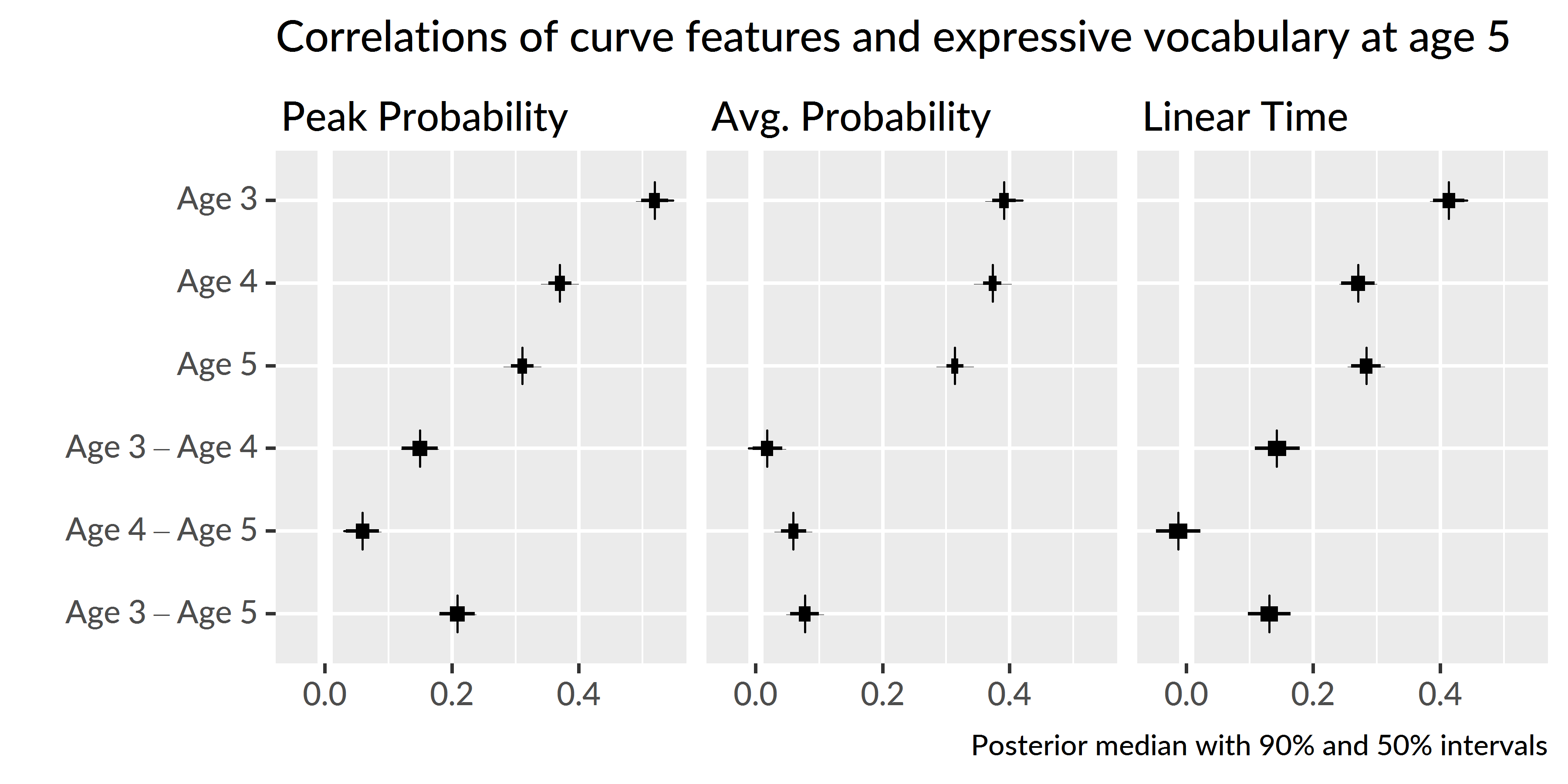
Figure 5.9: Uncertainty intervals for the correlations of growth curve features at each age with age-5 expressive vocabulary (EVT-2 standard scores). The bottom rows provide intervals for the pairwise differences in correlations between timepoints. For example, the top row of the left panel is the correlation between age-3 peak probability and age-5 expressive vocabulary.
Peak looking probabilities from age 3 were strongly correlated with age 4 receptive vocabulary, r = .62 [.61, .64], and this correlation was much greater than the correlation observed for the age 4 growth curve peaks, r3−4 = .26 [.23, .29]. The correlation for age 3 average looking probabilities, r = .45 [.44, .47], was greater than the age 4 correlation, r3−4 = .08 [.06, .11], and the correlation for age 3 linear time features, r = .51 [.49, .54], was likewise greater, r3−4 = .22 [.19, .26].
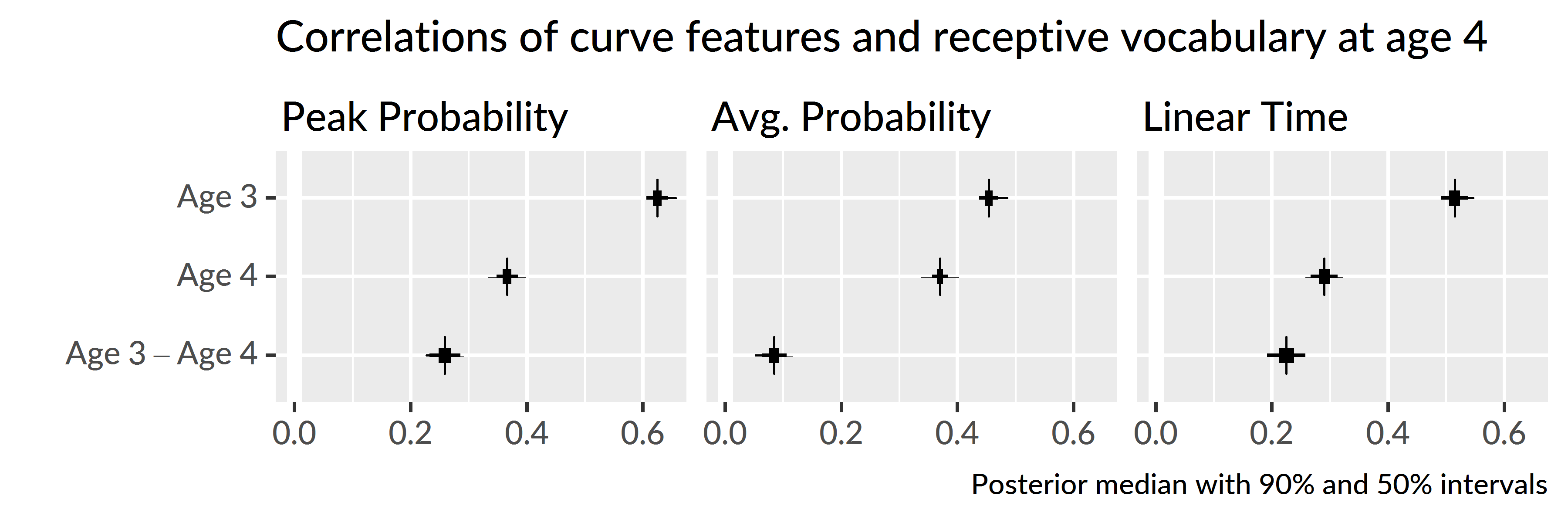
Figure 5.10: Uncertainty intervals for the correlations of growth curve features from age 3 and age 4 with age-4 receptive vocabulary (PPVT-4 standard scores). The bottom row shows pairwise differences between the age-3 and age-4 correlations.
Summary. Although individual differences in word recognition were stable over time, early differences were more significant than later ones. The strongest predictors of future vocabulary size were the growth curve features from age 3. Of these features, correlations were strongest for peak looking probabilities.
5.6 Discussion
In the preceding analyses, I examined many aspects of children’s recognition of familiar words. First, I modeled how children’s looking patterns on average changed year over year. Children’s word recognition improved each year: The growth curves grew steeper, reached higher peaks, and increased in their overall average value each year. This result was unsurprising, but it was valuable because it confirmed that this word recognition task scaled with development. The task was simple enough that children could recognize words at age 3 but challenging enough for children’s performance to improve each year.
After establishing how the averages changed each year, I next asked how variability changed each year. To tackle this question, I used posterior predictive inference to have the model simulate samples of data, and in particular, to simulate new participants. The range of performance narrowed each year, so that children were most variable at age 3 and least variable at age 5. This result is consistent with a model of development where children vary widely early on and converge on a more mature level of performance. From this perspective, word recognition is a skill where children “grow out” of immature and highly variable performance patterns. An alternative outcome would have been concerning: Word recognition differences that expanded with age with some children falling behind their peers.
Although the range of individual differences decreased with age, individual differences did not disappear over time. When children at each age were ranked using growth curve features, I found a high degree of correspondence among these ratings. Children who were faster or more accurate at age 3 remained relatively fast or accurate at age 5. Thus, differences in word recognition were longitudinally stable over the preschool years. Extrapolating forwards in time, these differences likely become smaller and smaller and become irrelevant for everyday listening situations. It is plausible, however, that under adverse listening conditions, individual differences might re-emerge and differentiate children’s word recognition performance.
Lastly, I analyzed how individual differences in word recognition features correlated with future vocabulary outcomes. The peak looking probabilities and growth curve slopes from age 3 showed the strongest correlations with future vocabulary scores. This finding was remarkable: Expressive vocabulary scores at age 5, for example, were more strongly correlated with word recognition data collected two years earlier than word recognition data collected during the same week.
We can understand the predictive value of age-3 word recognition performance from two perspectives. The first interpretation is statistical. Differences in children’s word recognition performance were greatest at age 3, so word recognition features at age 3 provide more variance and more information about the children and their future vocabulary size. The second interpretation is conceptual. Correlations were strongest for the growth curve peaks. We can think of this feature as measuring children’s maximum word recognition certainty. A child with a peak of .5, for example, looked the target image half of the time when they were most certain about the word. Although all of the words used were familiar to preschoolers, children with higher peaks knew those words better. These children had a stronger foundation for word-learning than children who show more uncertainty during word recognition, and as a result, these children had developed larger vocabularies two years later.
References
Barr, D. J. (2008). Analyzing ‘visual world’ eyetracking data using multilevel logistic regression. Journal of Memory and Language, 59(4), 457–474. doi:10.1016/j.jml.2007.09.002
Mirman, D., Dixon, J. A., & Magnuson, J. S. (2008). Statistical and computational models of the visual world paradigm: Growth curves and individual differences. Journal of Memory and Language, 59(4), 475–494. doi:10.1016/j.jml.2007.11.006
Mirman, D. (2014). Growth curve analysis and visualization using R. Boca Raton, FL: CRC Press/Taylor & Francis Group.
Oleson, J. J., Cavanaugh, J. E., McMurray, B., & Brown, G. (2017). Detecting time-specific differences between temporal nonlinear curves: Analyzing data from the visual world paradigm. Statistical Methods in Medical Research, 26(6), 2708–2725. doi:10.1177/0962280215607411
Seedorff, M., Oleson, J. J., & McMurray, B. (2018). Detecting when timeseries differ: Using the Bootstrapped Differences of Timeseries (BDOTS) to analyze Visual World Paradigm data (and more). Journal of Memory and Language, 102, 55–67. doi:https://doi.org/10.1016/j.jml.2018.05.004
Kruschke, J. K., & Liddell, T. M. (2017). The Bayesian New Statistics: Hypothesis testing, estimation, meta-analysis, and power analysis from a Bayesian perspective. Psychonomic Bulletin & Review, 1–29. doi:10.3758/s13423-016-1221-4
Gamer, M., Lemon, J., & Singh, I. F. P. (2012). irr: Various coefficients of interrater reliability and agreement. Retrieved from https://CRAN.R-project.org/package=irr
More generally, I think of there being a flexibility–interpretability tradeoff with additive models being the most flexible but having the least interpretable parameters, functional curves being the least flexible but having the most interpretable parameters, and polynomials falling in between the two.↩
My goals in using this method were simply to estimate model effects and quantify the uncertainty about those effects. This pragmatic, estimation-based approach of Bayesian statistics is illustrated in texts by Gelman and Hill (2007) and McElreath (2016).↩