Chapter 4 Method
4.1 Participants
The data were collected as part of a three-year longitudinal study.2 For convenience, I refer to the three years as age 3, age 4, and age 5, although the participants on average were three months younger than those nominal ages. In particular, the participants were 28–39 months-old at age 3, 39–52 at age 4, and 51–65 at age 5. Approximately, 180 children participated at age 3, 170 at age 4, and 160 at age 5. Of these children, approximately 20 were identified by their parents as late talkers. Prospective families were interviewed over telephone before participating in the study. Children were not scheduled for testing if a parent reported language problems, vision problems, developmental delays, or an individualized education program for the child. Recruitment and data collection occurred at two Learning to Talk lab sites—one at the University of Wisconsin–Madison and the other at the University of Minnesota.
Table 4.1 summarizes the cohort of children in each year of testing. The numbers and summary statistics here are general, describing children who participated at each year, but whose data may have been excluded from the analyses. Some potential reasons for exclusion include: excessive missing data during eyetracking, experiment or technology error, developmental concerns not identified until later in the study, or a failed hearing screening. Final sample sizes depend on the measures needed for an analysis and the results from data screening checks.
| Year 1 (Age 3) | Year 2 (Age 4) | Year 3 (Age 5) | |
|---|---|---|---|
| N | 184 | 175 | 160 |
| Boys, Girls | 94, 90 | 89, 86 | 82, 78 |
| Maternal ed.: Low, Mid, High | 15, 98, 71 | 12, 92, 71 | 6, 90, 64 |
| Dialect: MAE, AAE | 171, 13 | 163, 12 | 153, 7 |
| Parent-identified late talkers | 20 | 19 | 16 |
| Age (months): Mean (SD) | 33 (3) | 45 (4) | 57 (4) |
| Age (months): Range | 28–39 | 39–52 | 51–66 |
| EVT-2 standard: Mean (SD) | 115 (18) | 118 (16) | 118 (14) |
| PPVT-4 standard: Mean (SD) | 113 (17) | 120 (16) | — |
| GFTA-2 standard: Mean (SD) | 92 (13) | — | 91 (13) |
4.2 Visual World Paradigm
This experiment used a version of the Visual World Paradigm for word recognition experiments (Law, Mahr, Schneeberg, & Edwards, 2016). In eyetracking studies with toddlers, two familiar images are usually presented: a target and a distractor. This experiment is a four-image eyetracking task that was designed to provide a more demanding word recognition task for preschoolers. In this procedure, four familiar images are presented onscreen followed by a prompt to view one of the images (e.g., find the bell!). The four images include the target word (e.g., bell), a semantically related word (drum), a phonologically similar word (bee), and an unrelated word (swing). Figure 4.1 shows an example of a trial’s items. This procedure measures a child’s real-time comprehension of words by capturing how the child’s gaze location changes over time in response to speech.
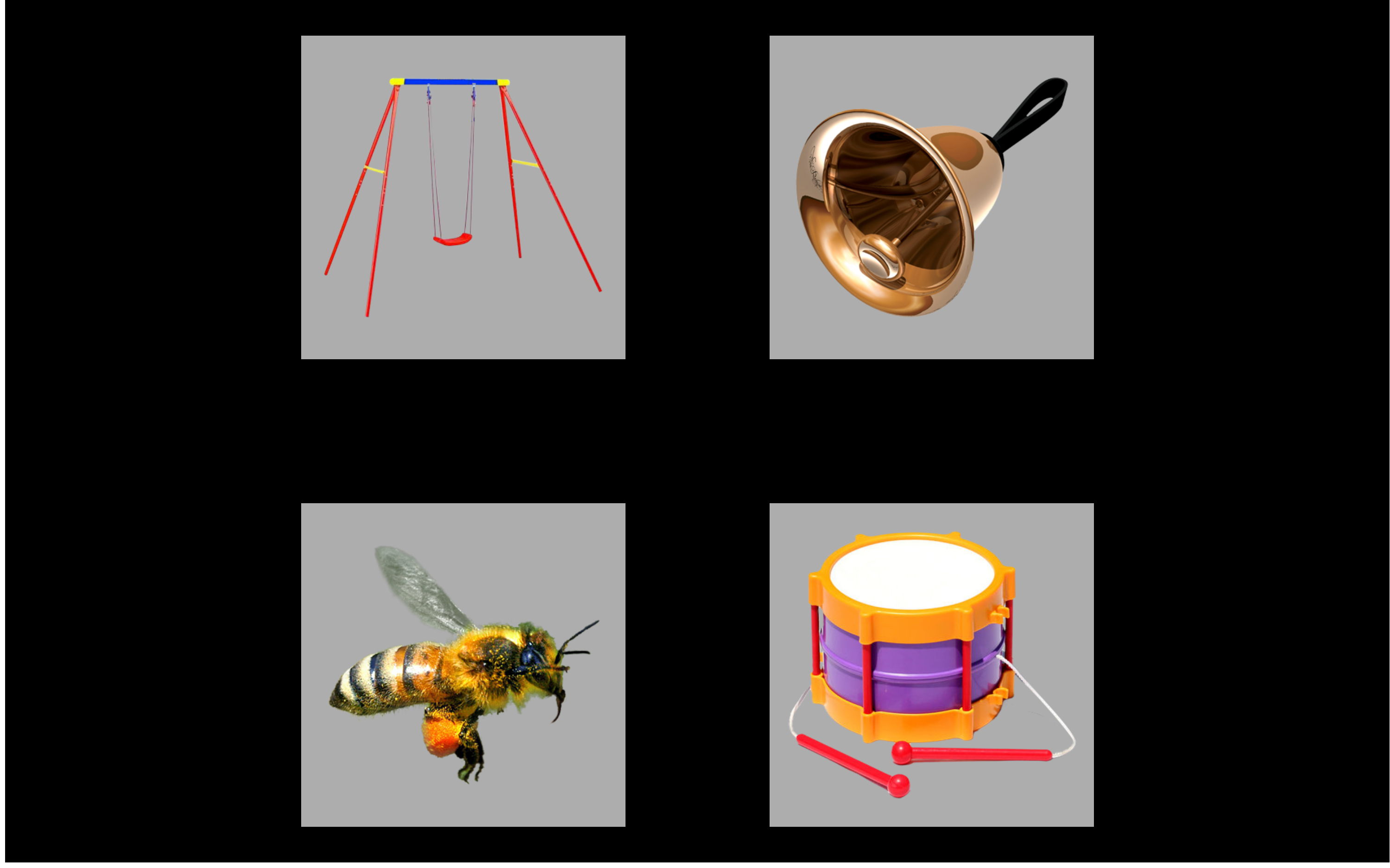
Figure 4.1: Example display for the target bell with the semantic foil drum, the phonological foil bee, and the unrelated swing.
This experimental design—an eyetracking study of word recognition with four images—is referred to as the Visual World Paradigm throughout the literature. See Huettig, Rommers, and Meyer (2011) for a historical review and an overview of how it has been used to study syntactic, pragmatic, semantic, and phonological processing. The paradigm has been used extensively to study word recognition in adult listeners—and in preschool-age children (Borovsky et al., 2012; Chow et al., 2017; Huang & Snedeker, 2011; Law et al., 2016).
4.3 Experiment administration
Children participating in the study were tested over two lab visits (on different dates). The first portion of each visit involved “watching movies”—that is, performing two blocks of eyetracking experiments. A play break or hearing screening occurred between the two eyetracking blocks, depending on the visit.
Each eyetracking experiment was administered as a block of trials (24 for this experiment and 36 for a two-image task—see Chapter 10). Children received two different blocks of each experiment. The blocks for an experiment differed in trial ordering and other features. Experiment order and block selection were counterbalanced over children and visits. For example, a child might have received Exp. 1 Block A and Exp. 2 Block B on Visit 1 and next received Exp. 2 Block A and Exp. 1 Block B on Visit 2. The purpose of this presentation was to control possible ordering effects where a particular experiment or block benefited from consistently occurring first or second.
Experiments were administered using E-Prime 2.0 and a Tobii T60XL eyetracker which recorded gaze location at a rate of 60 Hz. The experiments were conducted by two examiners, one “behind the scenes” who controlled the computer running the experiment and another “onstage” who guided the child through the experiment. At the beginning of each block, the child was positioned so the child’s eyes were approximately 60 cm from the screen. The examiners calibrated the eyetracker to the child’s eyes using a five-point calibration procedure (center of screen and centers of four screen quadrants). The examiners repeated this calibration procedure if one of the five calibration points for one of the eyes did not calibrate successfully. During the experiment, the behind-the-scenes examiner monitored the child’s distance from the screen and whether the eyetracker was capturing the child’s gaze. The onstage examiner coached the child to stay fixated on the screen and repositioned the child as needed to ensure the child’s eyes were being tracked. Every six or seven trials in a block of an experiment, the experiment briefly paused with a reinforcing animation or activity. During these breaks, the onstage examiner could reposition the child if necessary before resuming the experiment.
We used a gaze-contingent stimulus presentation. First, the images appeared in silence onscreen for 2 s as a familiarization period. The experiment’s software procedure then checked whether the child’s gaze was being recorded. If the procedure could continuously track the child’s gaze for 300 ms, the child’s gaze was verified and the trial continued. If the procedure could not verify the gaze after 10 s, the trial continued. This step guaranteed that for most trials, the child was looking to the display before presenting the carrier phrase and that the experiment was ready to record the child’s response to the carrier. During year 1 (age 3) and year 2 (age 4), an attention-getter (e.g., check it out!) played 1 s following the end of the target noun. These reinforcers were dropped in year 3 (age 5) to streamline the experiment for older listeners.
4.4 Stimuli
The four images on each trial consisted of a target noun, a phonological foil, a semantic foil, and an unrelated word. The phonological competitors shared a syllable onset (e.g., flag–fly, bell–bee), shared an initial consonant (bread–bear, swing–spoon), had a phonetically similar consonant onset (kite–gift), or shared a syllable rime (van–pan). The semantic competitors included words from the same category (e.g., shirt–dress, horse–bear), words that were perceptually similar (sword–pen, flag–kite), and words with less obvious relationships (van–horse, swan–bee). These different competitor types (phonological vs. semantic) and subtypes (e.g., shared syllable onset vs. rimes, shared category vs. perceptually similar) likely participate in word recognition to varying degrees and at different stages during lexical processing. For the analysis of familiar word recognition, I include all the competitors—they are aggregated together as distractors—but for the analysis of phonological and semantic competitors, I focus on subsets of competitors: the shared syllable onsets for phonological competitors and the category neighbors for semantic competitors. Appendix A provides a complete list of the items used in the experiment and in the analyses of competitor effects.
The stimuli were recorded in both Mainstream American English (MAE) and African American English (AAE), so that the experiment could accommodate the child’s home dialect. Prior to the lab visit, we made a preliminary guess about the child’s home dialect based on recruitment channel, address, and other factors. If we expected the dialect to be AAE, then the lab visit was led by an examiner who natively spoke AAE and could fluently dialect-shift between AAE and MAE. At the beginning of the lab visit, the examiner listened to the interactions between the child and caregiver in order to confirm the child’s home dialect. Prompts to view the target image of a trial (e.g., find the girl) used the carrier phrases “find the” and “see the”. These carriers were recorded in the frame “find/see the egg” and cross-spliced with the target nouns to minimize coarticulatory cues on the determiner “the”. The stimuli were re-recorded after the first year of the study with the same speakers so that the average durations of the two dialect versions were more similar.
The images used in the experiment consisted of color photographs on gray backgrounds. These images were piloted with 30 children from two preschool classrooms to ensure that children consistently used the same label for familiar objects. The two preschool classrooms differed in their students’ SES demographics: One classroom (13 piloting students) was part of a university research center which predominantly serves higher-SES families, and the other classroom (17 piloting students) was part of Head Start center which predominantly serves lower-SES families. The images were tested by presenting four images (a target, a phonological foil, a semantic foil and an unrelated word) and having the student point to the named image. The pictures were recognized by at least 80% of students in each classroom.
4.5 Data screening
To process the eyetracking data, I first mapped gaze x-y coordinates onto the onscreen images. I next performed deblinking. I interpolated short runs of missing gaze data (up to 150 ms) if the same image was fixated before and after the missing data run. Put differently, I classified a window of missing data as a blink if the window was brief and the gaze remained on the same image before and after the blink. I interpolated missing data from blinks using the fixated image.
After mapping the gaze coordinates onto the onscreen images, I performed data screening. I considered the time window from 0 to 2000 ms after target noun onset. I identified a trial as unreliable if at least 50% of the looks were missing during the time window. I excluded an entire block of trials if it had fewer than 12 reliable trials. The rationale for blockwise exclusion was that if the majority of trials were unreliable, then there was probably a problem during the session, such as a technical difficulty with the eyetracker or the child not complying with the task. As a result, all of the trials would be of questionable quality.
Table 4.2 shows the numbers of participants and trials at each year before and after data screening. There were more children in the second year than the first due to a timing error in the initial version of this experiment, leading to the exclusion of 27 participants from the first year.
| Dataset | Year | Children | Blocks | Trials | Percent Missing |
|---|---|---|---|---|---|
| Raw | Age 3 | 178 | 332 | 7967 | 24.4% |
| Age 4 | 180 | 347 | 8327 | 22.9% | |
| Age 5 | 163 | 322 | 7724 | 17.8% | |
| Screened | Age 3 | 163 | 291 | 5951 | 7.9% |
| Age 4 | 165 | 305 | 6421 | 8.5% | |
| Age 5 | 156 | 295 | 6483 | 7.8% | |
| Raw − Screened | Age 3 | 15 | 41 | 2016 | 16.5% |
| Age 4 | 15 | 42 | 1906 | 14.3% | |
| Age 5 | 7 | 27 | 1241 | 10.1% |
4.6 Model preparation
To prepare the data for modeling, I downsampled the data into 50-ms (3-frame) bins, reducing the eyetracker’s effective sampling rate to 20 Hz. Fixations have durations on the order of 100 or 200 ms, so capturing data every 16.67 ms oversamples eye movements and can introduce high-frequency noise into the signal. Binning together data from neighboring frames can smooth out this noise. I modeled the looks from 250 to 1500 ms. I chose this window after visualizing the observed fixation probabilities and identifying when during a trial the probabilities started to rise and later plateaued. Lastly, I aggregated looks by child, year and time, and created orthogonal polynomials to use as time features for the model. Orthogonal polynomials are described in the next chapter.
Figure 4.2 depicts each child’s proportion of looks to the target image following the data screening and model preparation steps. These are the observed or empirical growth curves; these are the probabilities that will be modeled with growth curve analysis. The lines start around .25 which is chance performance on four-alternative forced choice task. The lines rise as the word unfolds, and they peak and plateau around 1400 ms.
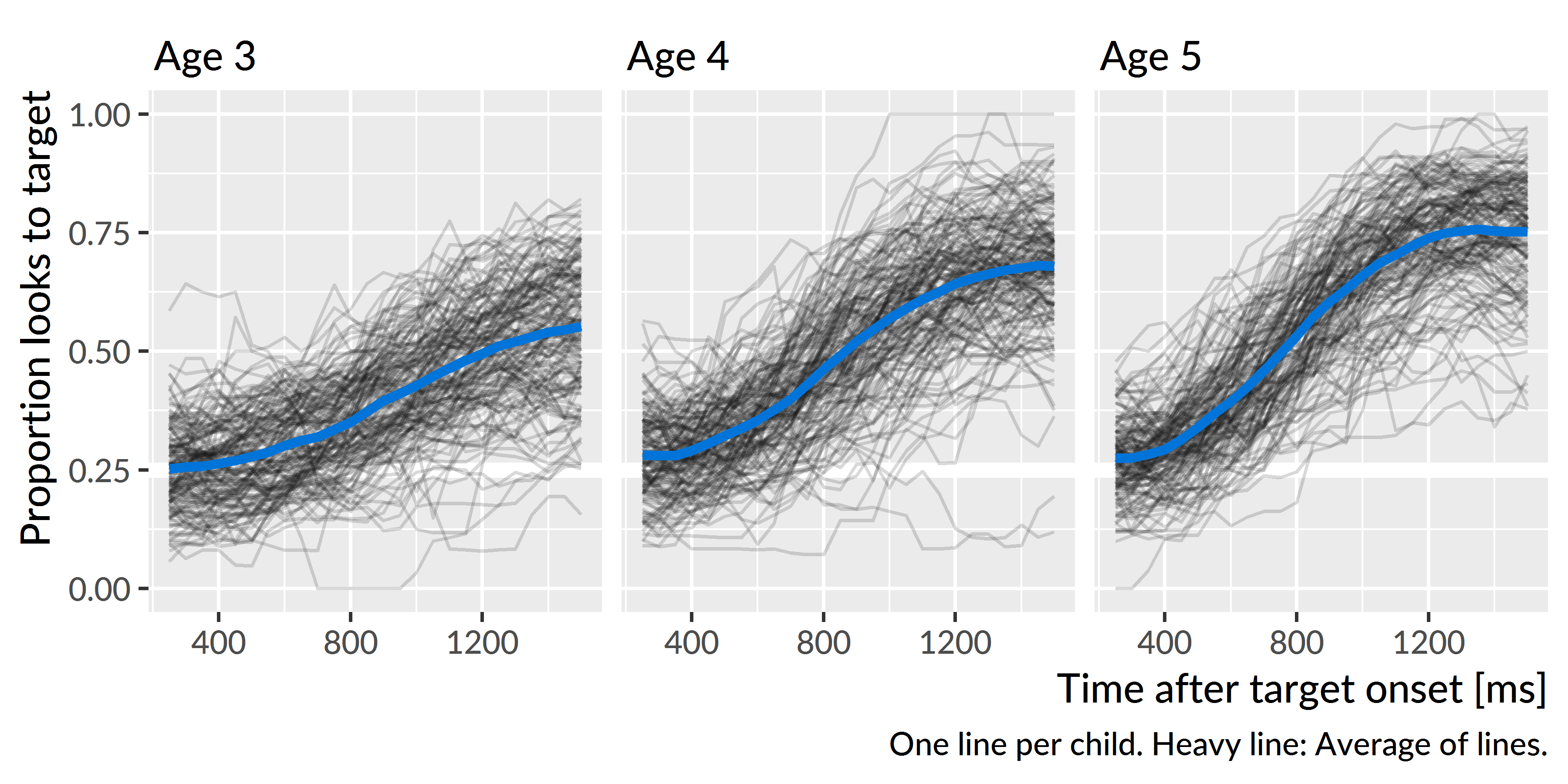
Figure 4.2: Empirical word recognition growth curves from each year of the study. Each line represents an individual child’s proportion of looks to the target image over time. The heavy lines are the averages of the lines for each year.
References
Law, F., II, Mahr, T., Schneeberg, A., & Edwards, J. R. (2016). Vocabulary size and auditory word recognition in preschool children. Applied Psycholinguistics. doi:10.1017/S0142716416000126
Huettig, F., Rommers, J., & Meyer, A. S. (2011). Using the visual world paradigm to study language processing: A review and critical evaluation. Acta Psychologica, 137(2), 151–171. doi:10.1016/j.actpsy.2010.11.003
Borovsky, A., Elman, J. L., & Fernald, A. (2012). Knowing a lot for one’s age: Vocabulary skill and not age is associated with anticipatory incremental sentence interpretation in children and adults. Journal of Experimental Child Psychology, 112(4), 417–436. doi:10.1016/j.jecp.2012.01.005
Chow, J., Aimola Davies, A. M., & Plunkett, K. (2017). Spoken-word recognition in 2-year-olds: The tug of war between phonological and semantic activation. Journal of Memory and Language, 93, 104–134. doi:10.1016/j.jml.2016.08.004
Huang, Y. T., & Snedeker, J. (2011). Cascading activation across levels of representation in children’s lexical processing. Journal of Child Language, 38(03), 644–661. doi:10.1017/S0305000910000206