Chapter 6 Effects of phonological and semantic competitors
6.1 Looks to the phonological competitor
The next question I asked was how children’s sensitivity to the phonological competitors changed over developmental time. Following our approach in Law et al. (2016), I only examined trials for which the phonological foil and the noun shared the same syllable onset. For example, this criterion included trials with dress–drum, fly–flag, or horse–heart, but it excluded trials kite–gift (phonetic feature difference), bear–bread (onset difference), and ring–swing (rimes). I kept 13 of the 24 trials. Appendix A provides a complete list of trials used.
The outcome measure for these analyses was the log-odds of fixating on the phonological competitor versus the unrelated word. Because children looked more to the target word with each year of the study, they necessarily looked less to the three distractors each year. Figure 6.1 illustrates how the proportions of looks to the phonological foils declined each year. Therefore, I examined the effect of the phonological foil in comparison to the unrelated foil. For example, on the trials where the target is fly, we can study the effect of the phonological foil flag by looking at when and to what degree the children fixate on flag more than the unrelated image pen. If a window of time of shows a consistent advantage for the phonological foil over the unrelated image, we conclude that the children were sensitive to the phonological foil during that window. By studying the time course of fixations to the phonological competitor versus the unrelated word, we can identify when the phonological competitor affected word recognition most significantly.
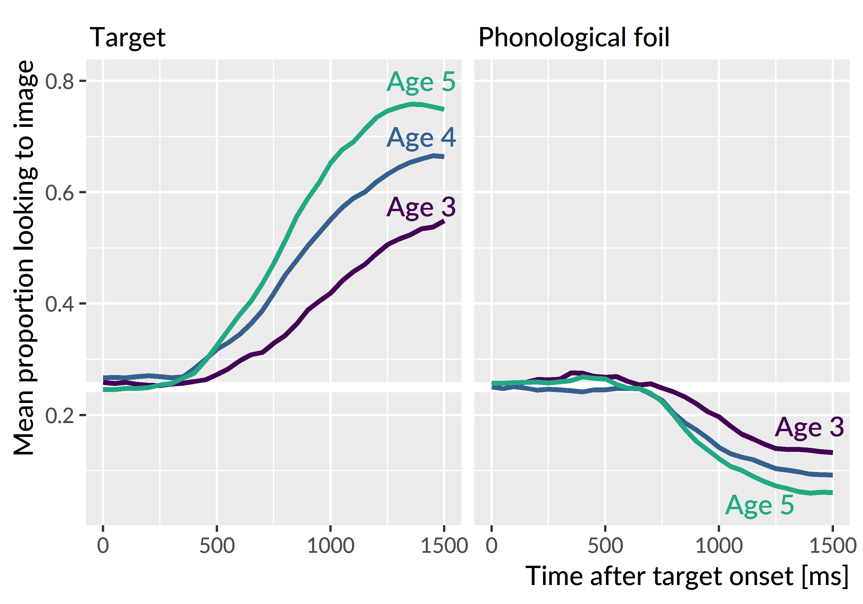
Figure 6.1: Because children looked more to the target as they grew older, they numerically looked less the foils too. This effect is why I evaluated the phonological and semantic foils by comparing them against the unrelated image.
As in the models from the previous chapter, I downsampled the data into 50-ms (3-frame) bins in order to smooth the data. For these trials, I modeled the looks from 0 to 1500 ms, and I aggregated looks by child, year and time bin. To account for the sparseness of the data, I used the empirical log-odds (or empirical logit) transformation (Barr, 2008). This transformation adds .5 to the looking counts. For example, a time-frame with 4 looks to the phonological foil and 1 look to the unrelated image has a conventional log-odds of log(4/1) = 1.39 and empirical log-odds of log(4.5/1.5) = 1.10. This transformation fills in bins with 0 looks with .5/.5 (avoiding 0/0 problems), and it dampens the extremeness of some probabilities that arise in sparse count data.
To model these data, I fit a generalized additive model with fast restricted maximum likelihood estimation (see Sóskuthy, 2017 for a tutorial for linguists; Winter & Wieling, 2016; Wood, 2017). Box 2 provides a brief overview of these models. I used the mgcv R package (vers. 1.8.24; Wood, 2017) with support from the tools in the itsadug R package (vers. 2.3; van Rij, Wieling, Baayen, & van Rijn, 2017).5 Appendix B contains the R code used to fit these models along with a description of the specifications represented by the model syntax.
Box 2: Intuition behind generalized additive models.
In these analyses, the outcome of interest is a value that changes over time in a nonlinear way. We model these time series by building a set of features to represent time values. In the growth curve analyses of familiar word recognition, I used a set of polynomial features which expressed time as the weighted sum of a linear trend, a quadratic trend and cubic trend. That is:
\[ \text{log\,odds}(\text{looking}) = \alpha + \beta_1\text{Time}^1 + \beta_2\text{Time}^2 + \beta_3\text{Time}^3 \]
But another way to think about the polynomial terms is as basis functions: A set of features that combine to approximate some nonlinear function of time. Under this framework, the model can be expressed as:
\[ \text{log\,odds}(\text{looking}) = \alpha + f(\text{Time}) \]
This is the idea behind generalized additive models and their smooth terms. These smooths fit nonlinear functions of data by weighting and adding simple functions together. The figures below show 9 basis functions from a “thin-plate spline” and how they can be weighted and summed to fit a growth curve.
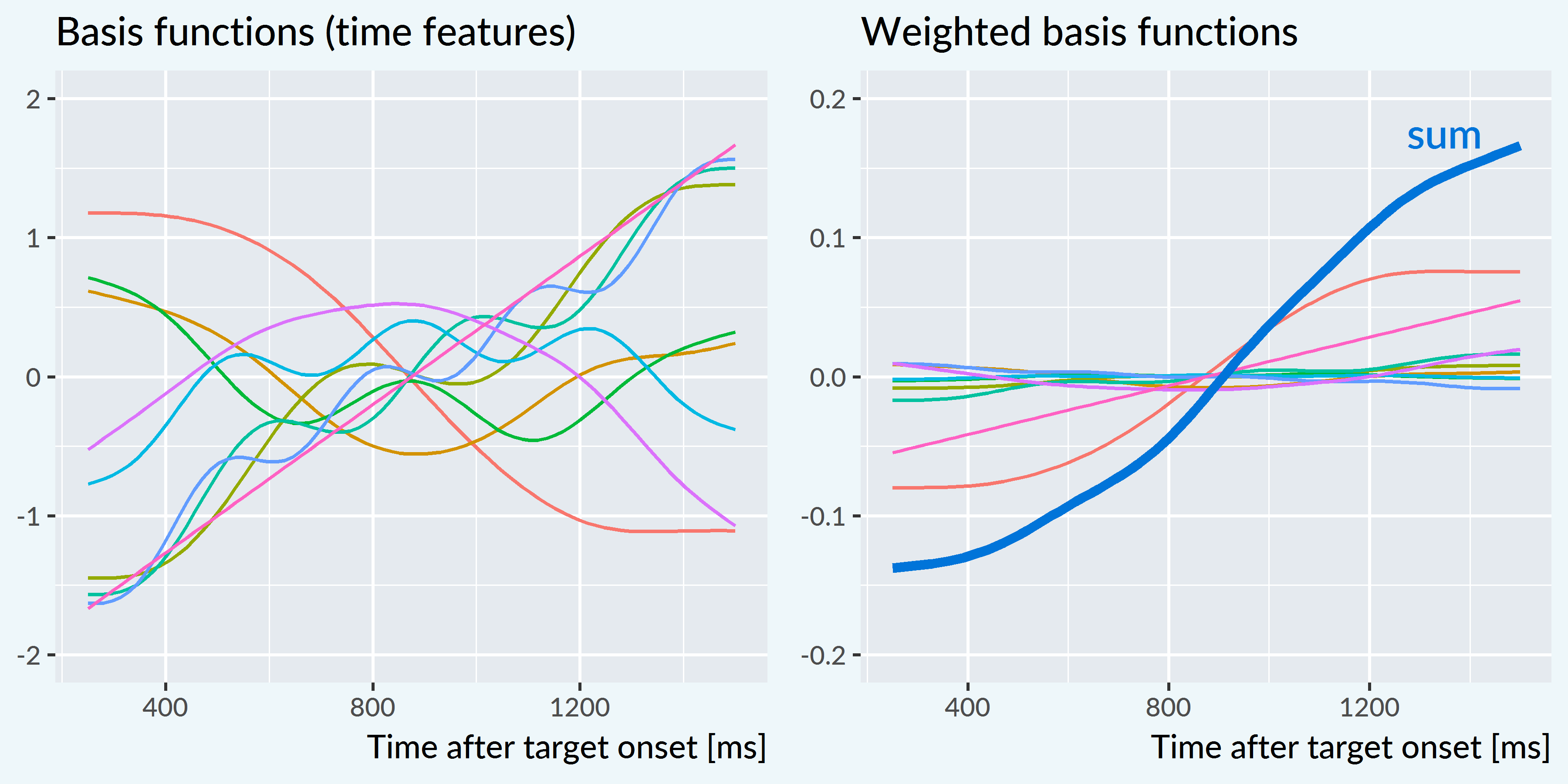
Each of these basis functions is weighted by a model coefficient, but the individual basis functions are not a priori meaningful. Rather, it is the whole set of functions that approximate the curvature of the data—i.e., f(Time)—so we statistically evaluate the whole batch of coefficients simultaneously. This joint testing is similar to how one might test a batch of effects in an ANOVA. If the batch of effects jointly improve model fit, we infer that there is a significant smooth or shape effect at play.
Smooth terms come with an estimated degrees of freedom (EDF). These values provide a sense of how many degrees of freedom the smooth consumed. An EDF of 1 is a perfectly straight line, indicating no smoothing. Higher EDF values indicate that the smooth term captured more curvature from the data.
The model included main effects of study year. These parametric terms work like conventional regression effects and determined the growth curve’s average values. The model used age 4 as the reference year, so the intercept represented the average looking probability at age 4. The year effects represented differences between age 4 vs. age 3 and age 4 vs. age 5.
The model also included smooth terms to represent the time course of the data. As with the parametric effects, age 4 served as the reference year. The model estimated a smooth for age 4 and it estimated difference smooths to capture how the curvature at age 3 and age 5 differed from the age-4 curvature. Each of these year-level smooths used 10 knots (9 basis functions). I also included child-level random smooths to represent child-level variation in growth curve shapes. Because there is much less data at the child level than at the year level, these random smooths only included 5 knots (4 basis functions). We can think of these simpler splines as coarse adjustments in growth curve shape to capture child-level variation from limited data. Altogether, the model contained the following terms:
\[ \small \begin{align*} \text{emp.\,log\,odds}(\text{phon. vs. unrelated}) =\ & \alpha + \beta_1\text{Age\,3} + \beta_2\text{Age\,5} +\ &\text{[growth curve averages]} \\ & f_1(\text{Time}, \text{Age\,4})\ + &\text{[reference smooth]} \\ & f_2(\text{Time}, \text{Age\,4} - \text{Age\,3})\ + &\text{[difference smooths]} \\ & f_3(\text{Time}, \text{Age\,4} - \text{Age\,5})\ + & \\ & f_i(\text{Time}, \text{Child}_i) &\text{[by-child random smooths]} \\ \end{align*} \normalsize \]
The model’s fitted values are shown in Figure 6.2. These are the average empirical log-odds of fixating on the phonological foil versus the unrelated image for each year of the study. The model captured the trend for increased looks to the competitor image with each year of the study. At age 4 and age 5, the shape rises from a baseline to the peak around 800 ms. These curves slope downwards and eventually fall beneath the initial baseline. The shape at age 3 does not have a steady rise from baseline and shows a small peak around 800 ms. The peak proportions of looks to the phonological competitor versus the unrelated word were .57 at 800 ms for age 3, .61 at 750 ms for age 4, and .64 at 750 ms for age 5.
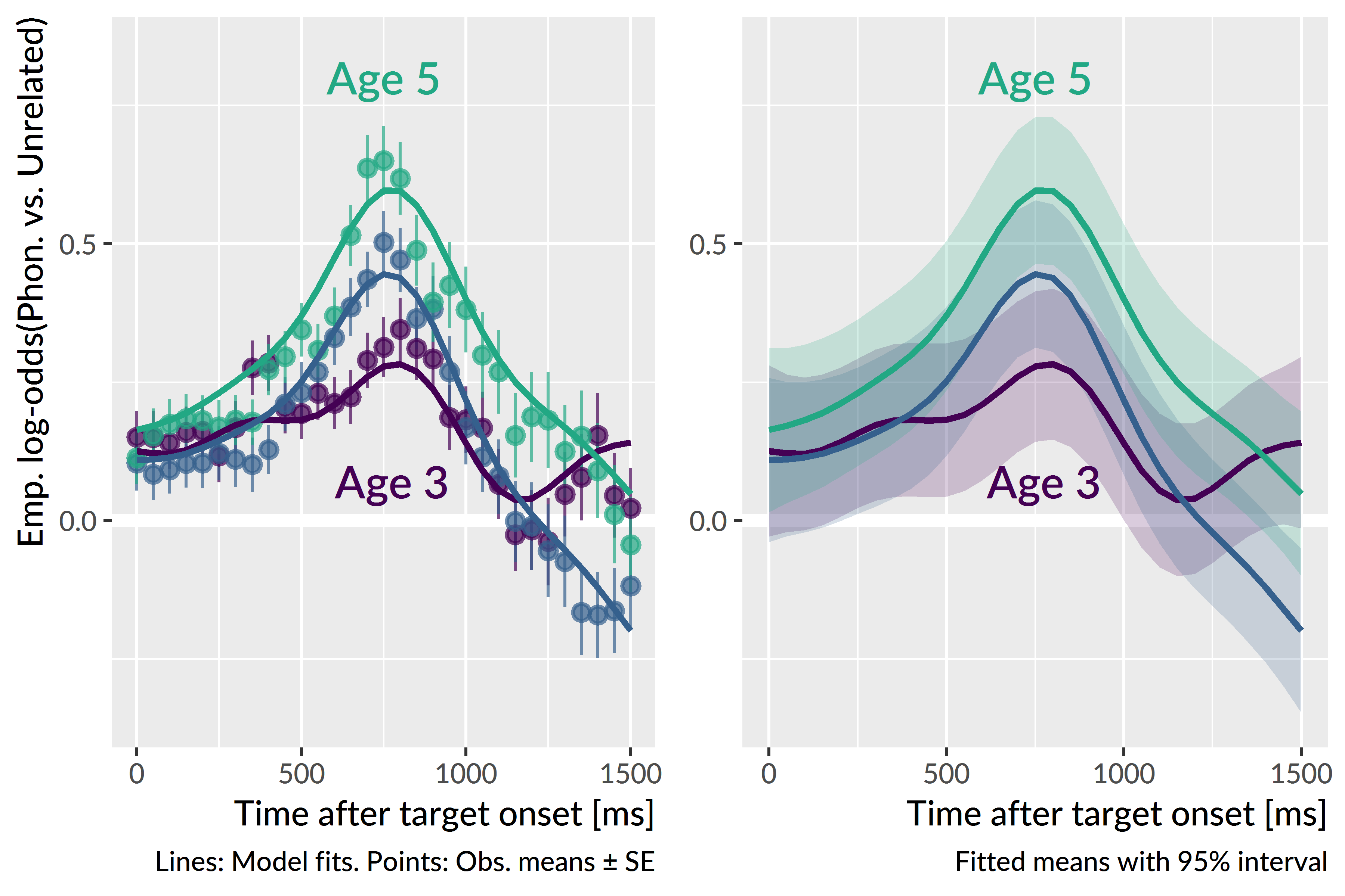
Figure 6.2: With each year of the study, children looked more to the phonological competitor (relative to the unrelated image) during and after the target noun. Both figures show means for each year estimated by the generalized additive model. The left panel compares model estimates to observed means and standard errors, and the right panel visualizes estimated means and their 95% confidence intervals.
The early peaks occur when one would expect if children are acting on partial phonological information. The similarity between the phonological competitor and the target noun occurs early on in the trial. Suppose a child acts on the first 400 ms of the phonological competitor. Assuming a 200–300 ms overhead to execute an eye movement in response to speech, the child would reach the phonological foil around 600–700 ms. This window is slightly before the observed peaks at 750–800 ms, but the age 4 and age 5 curves both are on the rise away from baseline during this window.
The average looks to the phonological foil over the unrelated image for age 4 was 0.16 emp. log-odds, .54 proportion units. The averages for age 3 and age 4 did not significantly differ, p = .85, but the average value was significantly greater at age 5, 0.31 emp. log-odds, .58 proportion units, p < .001. Visually, this effect shows up in the almost constant height difference between the age-4 and the age-5 curves.
There was a significant smooth term for time at age 4, estimated degrees of freedom (EDF) = 7.28, p < .001. Figure 6.3 visualizes how and when the smooths from other ages differed from the age-4 smooth.
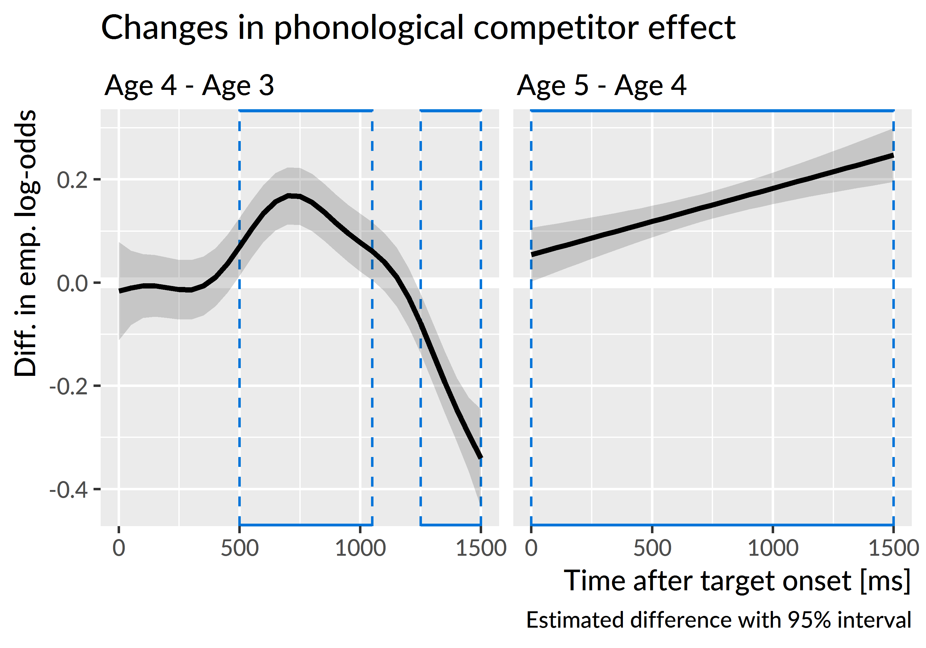
Figure 6.3: Differences in the average looks to the phonological competitor versus the unrelated image between age 4 and the other ages. Plotted line is estimated difference and the shaded region is the 95% confidence interval around that difference. Boxes highlight regions where the 95% interval excludes zero. From age 3 to age 4, children become more sensitive to the phonological foil during and after the target noun. The linear difference curve for age 4 versus age 5 indicates that the two years largely have the same curvature, but they steadily diverge over the course of the trial.
The age-3 and age-4 curves significantly differed, EDF = 5.48, p < .001. In particular, the curves are significantly different from 500 to 1050 ms. This result confirms that the looks to the phonological foil increased from age 3 and age 4 during the time window immediately following presentation of the noun and that children became more sensitive to the phonological similarities between the competitor and the target from age 3 to age 4.
The age-3 and age-4 curves also differed significantly after 1250 ms, so that at age 4 children looked less to the competitor compared to age 3. The effect reflects how the looks to phonological competitor decrease as a trial progresses. After an incorrect look to the foil, the children on average corrected their gaze and looked even less to the phonological foil. We do not observe this degree of correction during age 3, because children at age 3 looked less overall to the phonological foil early on.
The age-4 and age-5 smooths also significantly differed, EDF = 1.00, p < .001, although the low EDF values indicates that the shape of the difference was a flat line. Thus, the difference between the age-4 and age-5 smooths is driven primarily by the intercept difference and a linear diverging trend—that is, the distance between the two grows slowly over time. The same general curvature was observed for the two age smooths, suggesting the same general looking behavior at both time points: Children showed an early increase in looks to the phonological foil relative to the unrelated image but after receiving disqualifying information from the rest of the word, the looks to the phonological foil rapidly decrease. The primary difference between age-4 and age-5 is that the competitor effect becomes more pronounced at age 5.
Summary. Children looked more to the phonological competitor than the unrelated image early on in the trials. The advantage of the phonological competitor peaked on average around 800 ms after target onset, and the early timing indicates that children were shifting their gaze in response to the fleeting phonological similarity of the competitor to the target noun. The peak was small at age 3 but increased in height with each year of the study. Children became more sensitive to the phonological cohort competitors as they grew older.
6.2 Looks to the semantic competitor
I asked how children’s sensitivity to the semantic competitor changed as they grew older. As in Law et al. (2016), I only examined trials for which the semantic foil and the noun were part of the same category. For example, I included trials with bee–fly, shirt–dress, and spoon–pan, but I excluded trials where the similarity was perceptual (sword–pen) or too abstract (swan–bee). This criterion kept 13 of the 24 trials. Appendix A provides a complete list of trials used.
For these trials, I used the same modeling technique as the one used for phonological competitors: Generalized additive models with year effects and a time smooth, time-by-year difference smooths, and time-by-child random smooths. I modeled the looks from 250 to 1800 ms. This window was 300 ms longer than the one used for the phonological competitors in order to capture late-occurring semantic effects.
The model’s fitted values are shown in Figure 6.4. The average empirical log-odds of fixating on the semantic competitor versus the unrelated word increased with each year of the study. All three years show the same general time course of effects: Looks begin to increase from a baseline around 750 ms and peak around 1300 ms. The peak proportions of looks to the semantic competitor versus the unrelated word increased as children grew older: The peaks were .65 at 1400 ms for age 3, .68 at 1400 ms for age 4, and .71 at 1350 ms for age 5. Moreover, the semantic competitor shows a decisive advantage over the unrelated image at age 3, in contrast to the limited advantage of the phonological competitor at age 3.
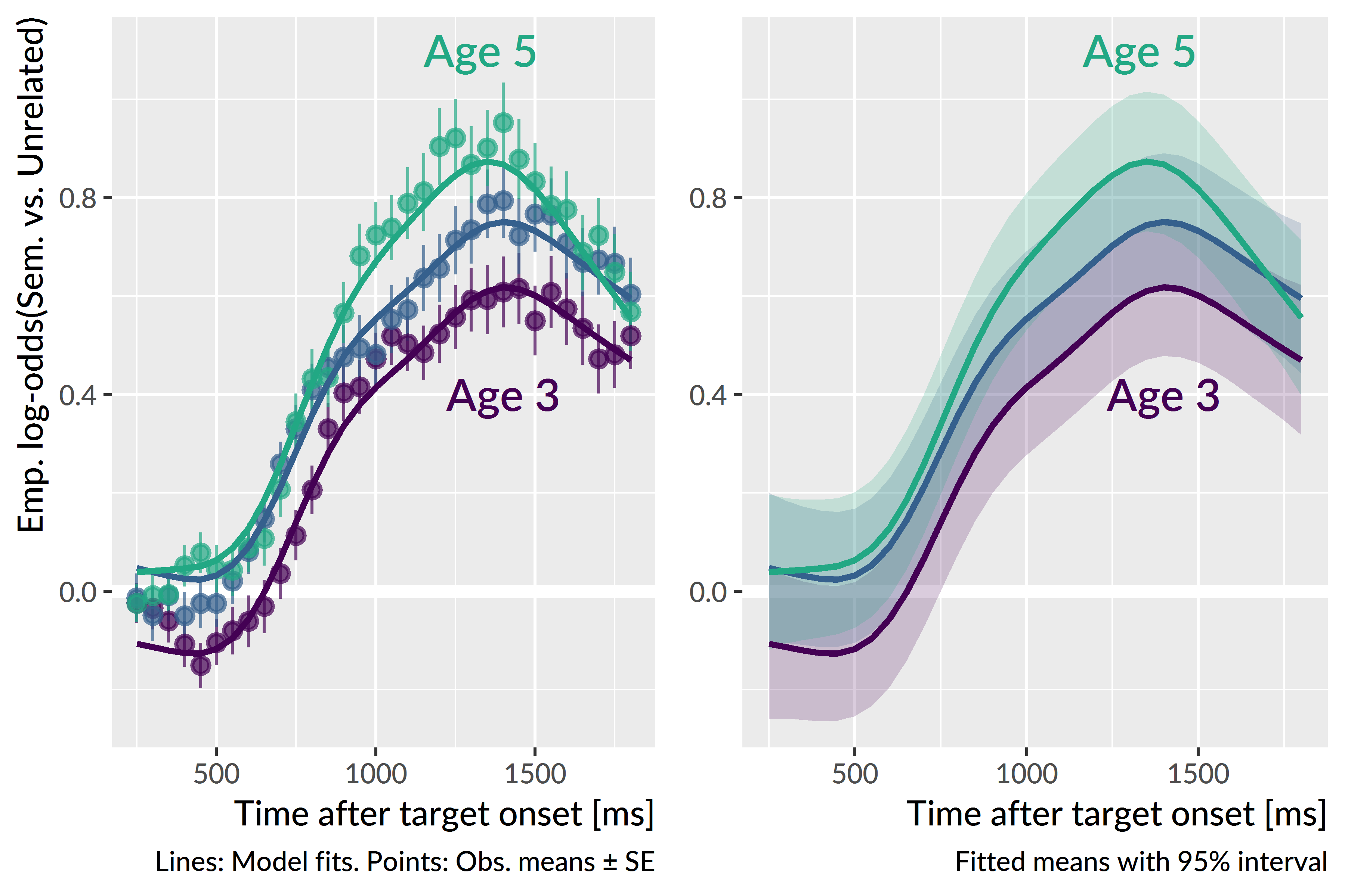
Figure 6.4: With each year of the study, children looked more to the semantic foil (relative to the unrelated image) with peak looking occurring after the target noun. Both figures show means for each year estimated by the generalized additive model. The left panel compares model estimates to observed means and standard errors, and the right panel visualizes estimated means and their 95% confidence intervals.
The average looks to the semantic foil over the unrelated image for age 4 was 0.44 emp. log-odds, .61 proportion units. Children looked significantly less to the semantic foil on average at age 3, 0.30 emp. log-odds, .57 proportion units, p < .001, and they looked significantly more to the semantic foil at age 5, 0.50 emp. log-odds, .62 proportion units, p < .001.
There was a significant smooth term for time at age 4, estimated degrees of freedom (EDF) = 7.04, p < .001. Figure 6.5 visualizes the time course of the differences between the smooths from each year.
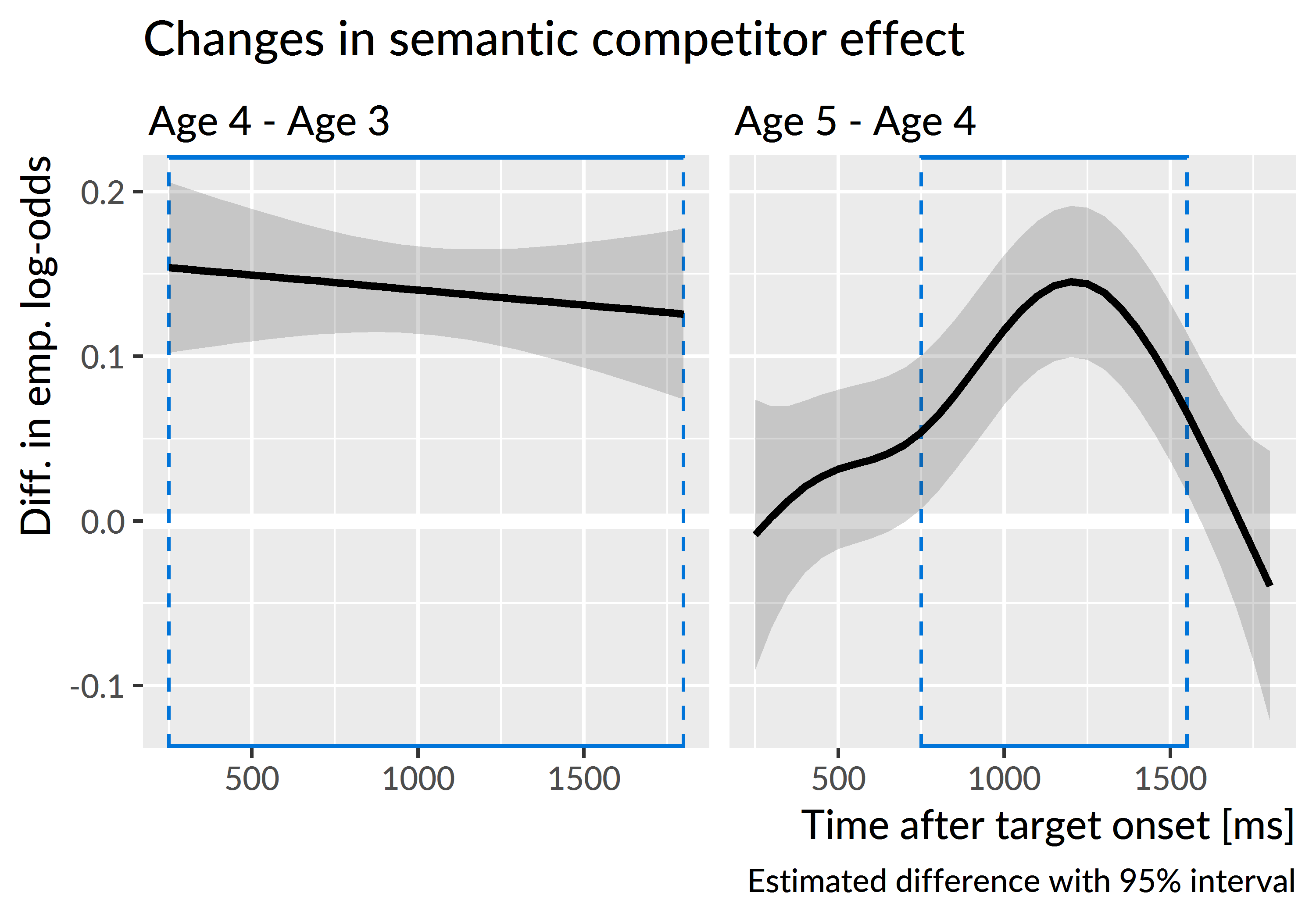
Figure 6.5: Differences in the average looks to the semantic competitor versus the unrelated word between age 4 and the other ages. Plotted line is estimated difference and the shaded region is the 95% confidence interval around that difference. Boxes highlight regions where the 95% interval excludes zero. The flat line on the left reflects how the shape of the growth curves remained the same from age 3 to age 4 and only differed in average height. From age 4 to age 5, the lines quickly diverge and the age-5 curve reaches a higher peak value.
The shapes of the age-3 and age-4 curves did not significantly differ, EDF = 1.00, p = .535. The age-3 curve begins to rise about 100 ms later, and it reaches a shallower peak value than the age-4 curve. These two features create a nearly constant height difference between the two curves, and thus the two curves show the same overall shape.
The age-4 and age-5 smooths significantly differed, EDF = 3.74, p < .001. The differences are greatest after the end of the target noun, in the window from 750 to 1500 ms. The two curves start from a similar baseline but quickly diverge as the age-5 curve reaches a higher peak value. After 1500 ms, the age-5 curve turns downwards to overlap with the age-4 curve. Children looked more to the semantic foil relative to the unrelated image, but they were also quicker to correct and look away from it.
Summary. Children became more sensitive to the semantic competitor, compared to the unrelated word, with each year of the study. The semantic foils clearly influenced looking patterns at age 3, in contrast to the muted effect observed for the phonological foils. The semantic effect also occurred when we would expect: After the end of the target noun, following the lexical activation of the target noun and its semantic neighbors.
6.3 Child-level differences in competitor sensitivity at age 3
Next, I asked whether children differed reliably in their sensitivity to the phonological and semantic foils based on speech perception and vocabulary measures collected at age 3.
As a measure of speech perception, I used scores from a minimal pair discrimination experiment administered during the first year of the study. The task (based on Baylis, Munson, & Moller, 2008) is essentially an ABX discrimination task: A picture of a familiar object is shown and labeled (e.g., “car”), another object is shown and labeled (“jar”), and then both images are shown and one of the two is named. The child then indicated which word they heard by tapping on the image on a touch-screen.
I derived speech perception scores by fitting a hierarchical item-response model. This logistic regression model estimates the probability of child i correctly choosing word j on word-pair k. The equation below provides a term-by-term description of the model. The model’s intercept term represents the average participant’s probability of correctly answering for an average item. By-child random intercepts capture a child’s deviation from the overall average, so they estimate the child’s ability. By-word and by-word-in-pair random intercepts capture the relative difficulty of particular items on the experiment. The by-word-in-pair effects were necessary because four words appeared in more than one word pair (e.g., juice–goose and juice–moose). The model also controlled for the children’s ages and receptive vocabulary scores (PPVT-4 growth scale values). These predictors were transformed to have mean 0 and standard deviation 1, so the model’s intercept reflected a child of an average age and an average vocabulary level. Therefore, the by-child intercepts reflect a child’s ability after controlling for age and receptive vocabulary.
\[ \small \begin{align*} \text{log\,odds}(\text{choose target}) =\ & \alpha\ + &\text{[average child ability]} \\ & \alpha_i\ + &\text{[difference of child}\ i \text{'s ability from average]} \\ & \alpha_j\ + &\text{[word}\ j\text{'s difficulty]} \\ & \alpha_{j,k}\ + &\text{[word}\ j \text{'s difficulty in word-pair}\ k] \\ & \beta_{1}\text{Age}\ + &\text{[child-level predictors]} \\ & \beta_{2}\text{Vocabulary} & \\ \end{align*} \normalsize \]
I tested whether phonemic discrimination ability at age 3 predicted looks to the phonological competitor over the unrelated image by modifying the generalized additive model from earlier. In particular, I included a smooth term for the phonemic discrimination ability score and a “smooth interaction” between the smooth of time and phonemic ability. These smooth interaction terms are analogous to interaction terms in linear models. In this case, the interaction term allows the ability score to change the shape of the time trend. The additive model was therefore:
\[ \small \begin{align*} \text{emp.\,log\,odds}(\text{phon. vs. unrelated}) =\ & \alpha\ +\ &\text{[growth curve average]} \\ & f_1(\text{Time})\ + &\text{[time smooth]} \\ & f_2(\text{Ability})\ + &\text{[ability smooth]} \\ & f_3(\text{Time} * \text{Ability})\ + &\text{[interaction smooth]} \\ & f_i(\text{Time}, \text{Child}_i) &\text{[by-child random smooths]} \\ \end{align*} \normalsize \]
The model included data from 144 participants; these were children with eyetracking data, receptive vocabulary and phonemic discrimination data at age 3. There was not a significant smooth effect for discrimination ability, EDF = 1.00, p = .551 or for an interaction smooth between time and ability, EDF = 8.37, p = .303.
To test the role of receptive vocabulary, I also fit analogous models using growth scale value scores from the PPVT-4, a receptive vocabulary test. I first adjusted these scores in a regression model to control for–that is, to partial out the effects of—age and predicted accuracy on the discrimination task. There was not a significant smooth effect for receptive vocabulary, EDF = 1.00, p = .868, or a significant interaction smooth between time and receptive vocabulary, EDF = 5.57, p = .610. Receptive vocabulary therefore was not related to looks to the phonological foil at age 3.
I tested the same two predictors on looks to the semantic foil at age 3. These child-level factors did not show any significant parametric effects, smooth effects or smooth interactions with time. Thus, children’s looks to the semantic foil were not reliably related to phonemic discrimination or receptive vocabulary.
Summary. These models tested whether two child-level factors—minimal-pair discrimination ability and receptive vocabulary—predicted looks to the phonological and semantic competitors at age 3. No significant effects were observed for all cases.
6.4 Discussion
In the preceding analyses, I examined children’s fixation patterns to the phonological and semantic competitors and how these fixation patterns changed over developmental time. With each year of the study, children looked more to the target overall, so they consequently looked less to the competitor images each year. To account for this fact, these analyses examined the ratio of looks to the competitors versus the unrelated word. This ratio measured the relative advantage of a competitor over the unrelated word.
6.4.1 Immediate activation of phonological neighbors
Developmentally, children became more sensitive to the phonological competitors with each year of the study. These words shared the same syllable onset as the target noun—for example, the pairs dress–drum or fly–flag. The competitors affected word recognition early on, with relative looks to the phonological foils peaking around 800 ms. The target nouns were approximately 800 ms in duration at age 3 and 550–800 ms at later ages. Assuming a 200–300 ms overhead for executing an eye movement in response to speech, this timing indicates that children shifted their gaze immediately, based on partial information. Moreover, the tendency to act on partial information became stronger with age, because the early advantage of the phonological competitor increased with each year of the study.
When children looked to the phonological competitor, they fixated on the wrong image and had to revise their interpretation of the noun. At ages 4 and 5, the early peaks of looks to the phonological competitor were followed by a steep, monotonic decrease in looks: Children rejected their initial interpretation of the word and considered other images. At age 3, the average pattern showed more wiggliness, suggesting that children were less decisive in rejecting the phonological competitor. The shapes of the looking patterns at age 4 and age 5 were essentially the same. In particular, the older children were not any faster in the rejecting the phonological competitor on average.
We can interpret these findings in terms of lexical processing dynamics. Under this view, incoming speech activates phonetic and phonemic and lexical representations. The word with the strongest activation is the favored interpretation and the object of the child’s fixations. The early looks to the phonological competitors reflect immediate activation of lexical units: Children activate words on the basis of partial acoustic information. This result is a hallmark of spoken word recognition. The activation of phonologically plausible words becomes stronger with age, as reflected in children’s increasing sensitivity to the phonological competitors. Some mechanisms that may explain this developmental pattern include changes in lexical organization so that neighborhoods of phonologically similar words coactivate and changes in lexical representation so that partial information can more eagerly activate compatible words.6
Children at age 4 and age 5 did not show any changes in how quickly they rejected the phonological foil, and this result suggests that lexical inhibition may not change over the preschool years. The reasoning is as follows: If children developed stronger lexical inhibition with age, so that lexical competition resolves more quickly, then we would expect activation of the phonological competitors to decay more quickly and for children to reject the phonological competitor more quickly. But this pattern is not what we observed in the growth curve analyses.7 The developmental trajectory here is one of increased activation, of children learning words and learning similarities among them so that phonological similar words participate in word recognition.
6.4.2 Late activation of semantic neighbors
The semantic competitors were from the same category as the target noun: for example, bee–fly or shirt–dress. Children showed year-over-year increases in their sensitivity to the semantic competitor, compared to the unrelated image. Looks the semantic foils started rising steadily 500–700 ms after target onset and peaked late in the trial, around 1300 ms. This time-course is more protracted than the immediate peaks observed for the phonological competitor.
In terms of lexical processing, this late timing is consistent with cascading activation: Spoken words immediately activate phonological neighborhoods with activation cascading onto semantically related words. As a particular word is favored, its semantic relatives receive more secondary activation. For example, children hear “find the shirt”, activate the target shirt, but also activate other pieces of clothing including dress. The late timing of looks to the semantic competitor therefore reflects late, secondary activation of the spoken word’s semantic relatives. In other words, the activation of a semantic neighbor (like dress) is greatest when the activation of the spoken word (shirt) is greatest which happens relatively late, once the competition among phonological alternatives resolves.
Under this account, children hear a word, activate it, and become increasingly likely to fixate on the semantic competitor, compared to the unrelated image. The late looks probably reflect a combination of behaviors: children considering the semantically related image to check their initial interpretation as well as children looking to the wrong image because of confusion, lack of knowledge, overriding activation from the semantic competitor, or lack of interest in the target.
Initially, I had subscribed to a confusion or lack-of-knowledge interpretation of the semantic competitor’s advantage. That is, children look to the semantic competitor because they do not know the difference between the target and the semantic competitor. After all, my thinking went, these were young children and decisions like bee vs. fly or goat vs. sheep can be difficult. But there are two objections to that line of reasoning. First, our lab piloted the set of words in preschool classrooms, so we confirmed that children could reliably and correctly point to bee even when fly is an alternative. Second, we would a priori expect that children’s confusion among words to be greatest when they are youngest and have much less experience with these semantic categories. (Indeed, children at age 3 looked less to the target overall, so in general, they were less successful at recognizing the target word.)
The late looks to the semantic competitor, relative to the unrelated image, however, were greatest at age 5. Children’s looks became more selective with age: They looked more to the semantic competitor because they had discovered the semantic connections among words. They had learned the similarity between bee and fly or shirt and dress. Put another way, to demonstrate confusion between two choices, children must learn some association that connects the two; they must use or activate some information that induces warranted uncertainty. Rather than confusion about the meaning of nouns, the late looks likely reflect a confirmatory behavior where children give some consideration to the semantic alternative. This is especially the case at age 5, where the advantage of semantic competitor quickly decreases after its peak, indicating rejection of the semantic competitor.
6.4.3 Lexical competitors and child-level predictors
I asked whether offline child-level measures predicted sensitivity to the phonological and semantic competitors at age 3. I used children’s ability scores from a minimal-pair discrimination task as a measure of phonemic speech perception, and I also used scores from a receptive vocabulary test. For the phonological competitor, I expected that children with better phonemic discrimination would show increased looks to the phonological competitor because they had more detailed phonemic representations that would activate phonological neighborhoods more quickly. For the semantic competitor, I likewise expected children with larger receptive vocabularies to show increased looks to the semantic competitor because these children knew more words and likely developed more semantic connections among the words. I tested these effects by using the scores as parametric effects to see if they predicted average looks to the competitor, and alternatively, by using the scores for smooth effects to see if they influenced the time course of looks to the foils.
None of these expectations held: Neither of the child-level measures predicted average sensitivity to the phonological or semantic competitors at age 3. Part of the result may be artifactual: The data—looks to a subset of images on a subset of trials—may be too limited at the individual level for the models to pick up on child-level effects. Part of the result may be developmental too: Children were least sensitive to the competitors at age 3, so individual differences may be too small for the data or models to capture. Further work, with different experimental designs, may elaborate on whether offline measures can reliably detect differences in sensitivity to lexical competitors during word recognition.
References
Law, F., II, Mahr, T., Schneeberg, A., & Edwards, J. R. (2016). Vocabulary size and auditory word recognition in preschool children. Applied Psycholinguistics. doi:10.1017/S0142716416000126
Barr, D. J. (2008). Analyzing ‘visual world’ eyetracking data using multilevel logistic regression. Journal of Memory and Language, 59(4), 457–474. doi:10.1016/j.jml.2007.09.002
Sóskuthy, M. (2017). Generalised additive mixed models for dynamic analysis in linguistics: a practical introduction. Retrieved from http://arxiv.org/abs/1703.05339
Winter, B., & Wieling, M. (2016). How to analyze linguistic change using mixed models, growth curve analysis and generalized additive modeling. Journal of Language Evolution, 1(1), 7–18. doi:10.1093/jole/lzv003
Wood, S. N. (2017). Generalized additive models: An introduction with R (2nd ed.). Boca Raton, FL: CRC Press/Taylor & Francis Group.
van Rij, J., Wieling, M., Baayen, R. H., & van Rijn, H. (2017). itsadug: Interpreting time series and autocorrelated data using GAMMs.
Baylis, A. L., Munson, B., & Moller, K. T. (2008). Factors affecting articulation skills in children with velocardiofacial syndrome and children with cleft palate or velopharyngeal dysfunction: A preliminary report. The Cleft Palate-Craniofacial Journal, 45(2), 193–207. doi:10.1597/06-012.1
Initially, I tried to use Bayesian polynomial growth curve models, as in the earlier analysis of the looks to the target image. These models however did not converge, even when strong priors were placed on the parameters. In principle, I could have used Bayesian generalized additive models, but the software ecosystem and available tools for model criticism and inference are currently rather limited.↩
I am not too committed to any particular mechanisms of representation or organization. Under a connectionist framework with distributed representations, for instance, a word is represented as a pattern of activation distributed over many shared units. (I think of numbers on a digital clock where seven lines turn on or off to make ten digits but exponentially more complicated.) In that case, representation and organization are inseparable, and it would make more sense to talk about the strength and number of connections instead. My point here is that the lexical mechanisms involved should be ones that enable stronger immediate activations as a result of learning more words.↩
Granted, there might be some subtle nonlinear effect at play where higher peak activations require a greater degree of inhibition to overcome, so changes in inhibition could be a plausible part of the developmental story. But there is no compelling reason from the data to make that assertion.↩