D Computational details for Study 2
D.1 Real words versus nonwords growth curves
These models were fit in R (vers. 3.5.0; R Core Team, 2018) with the brms package (vers. 2.3.1; Bürkner, 2017).
The orthogonal polynomial features for Time, they were scaled as in Study 1, so that the linear feature ranged from −.5 to .5. Under this scaling a unit change in Time1 was equal to change from the start to the end of the analysis window.
The model formula used to specify the model with brms is printed below. The variables ot1, ot2, and ot3 are the polynomial time features, ResearchID identifies children, and Condition identifies the experimental condition (either, the nonword or real word condition). Target counts the number of looks to the target image at each time bin; trials() is a flag that tells brms the number of trials for the binomial process. Here, it is the variable Trials, which is equal to the number of looks to target and distractor in each bin. The syntax (1 + ot1 + ot2 + ot3) * Condition specifies a Time x Condition interaction; it says to estimate an intercept and the three time feature effects for each condition. The line (ot1 + ot2 + ot3 | ResearchID/Condition) describes the random-effect structure of the model with the / indicating that data from each Condition is nested within each ResearchID.
library(brms)

# Fit a hierarchical logistic regression model
formula <- bf(
  Target | trials(Trials) ~
    (1 + ot1 + ot2 + ot3) * Condition +
    (1 + ot1 + ot2 + ot3 | ResearchID/Condition),
  family = binomial)
The priors for the model are specified below. The regression effects (class = "b") have a prior of Normal(0, 1). Because most of the action in the growth curves is a sharp rise, the linear time effect ot1 has a slightly wider prior of Normal(0, 2). These priors are uninformative in terms of direction–both positive and negative effects are equally likely–but they are informative in terms of magnitude. A weakly informative LKJ(2) prior is put on the random-effect correlations. I review the role of the LKJ prior in Appendix B. A weakly informative prior is put on the random-effect standard deviations Student-t([df] 7, [mean] 0, [sd] 3). The Student-t distribution is like the normal distribution but it provides slightly thicker tails which allow extreme or outlying values.
priors <- c(
  # Population-average intercept
  set_prior(class = "Intercept", "normal(0, 1)"),
  # Population-average slopes
  set_prior(class = "b", "normal(0, 1)"),
  # ... expect somewhat larger range of effects for linear time
  set_prior(class = "b", coef = "ot1", "normal(0, 2)"),
  # Correlations for random effect terms
  set_prior(class = "cor", "lkj(2)"),
  # Standard deviation of the distribution from
  # which random-intercepts are drawn
  set_prior(class = "sd", "student_t(7, 0, 3)"))
I originally tried a single model containing all three years with corresponding year effects, year × time interactions, and year × condition × time interactions, but this model took 30 hours to run and did not converge. Therefore, I fit separate models for each year of the study using syntax like the following.
m_age3 <- brm(
  formula = formula,
  data = d_age3,
  prior = priors,
  chains = 4,
  iter = 2000,
  cores = 4,
  control = list(adapt_delta = .99))

# Save the output
readr::write_rds(m_age3, "age3_mp.rds.gz")
This code fits the model using four sampling chains in parallel over four processing cores. Early attempts at the model produced warnings, so I increased the adapt_delta control option to make the sampling more robust and eliminate the warnings.
Model summary for real words versus nonwords at age 3:
m1 <- readr::read_rds("./data/aim2-real-vs-nw-tp1.rds.gz")
summary(m1, priors = TRUE, prob = .9)
#>  Family: binomial
#>   Links: mu = logit
#> Formula: Target | trials(Trials) ~
#>            (ot1 + ot2 + ot3) * Condition +
#>            (ot1 + ot2 + ot3 | ResearchID/Condition)
#>    Data: test_data_1 (Number of observations: 7450)
#> Samples: 4 chains, each with iter = 2000; warmup = 1000; thin = 1;
#>          total post-warmup samples = 4000
#>
#> Priors:
#> b ~ normal(0, 1)
#> b_ot1 ~ normal(0, 2)
#> Intercept ~ normal(0, 1)
#> L ~ lkj_corr_cholesky(2)
#> sd ~ student_t(7, 0, 3)
#>
#> Group-Level Effects:
#> ~ResearchID (Number of levels: 149)
#>                    Estimate Est.Error l-90% CI u-90% CI Eff.Sample Rhat
#> sd(Intercept)          0.73      0.13     0.51     0.93        290 1.00
#> sd(ot1)                0.64      0.40     0.05     1.31         68 1.03
#> sd(ot2)                0.34      0.19     0.04     0.65        130 1.02
#> sd(ot3)                0.14      0.10     0.01     0.33        233 1.01
#> cor(Intercept,ot1)     0.25      0.33    -0.36     0.72        176 1.02
#> cor(Intercept,ot2)    -0.26      0.32    -0.73     0.32        838 1.00
#> cor(ot1,ot2)          -0.08      0.37    -0.64     0.56        380 1.01
#> cor(Intercept,ot3)     0.12      0.34    -0.47     0.65       1338 1.00
#> cor(ot1,ot3)           0.06      0.38    -0.57     0.66        740 1.00
#> cor(ot2,ot3)          -0.01      0.37    -0.60     0.61       1226 1.00
#>
#> ~ResearchID:Condition (Number of levels: 298)
#>                    Estimate Est.Error l-90% CI u-90% CI Eff.Sample Rhat
#> sd(Intercept)          1.24      0.08     1.12     1.37        611 1.00
#> sd(ot1)                2.66      0.16     2.40     2.93        320 1.01
#> sd(ot2)                1.40      0.09     1.25     1.55        572 1.00
#> sd(ot3)                0.83      0.05     0.74     0.92        923 1.00
#> cor(Intercept,ot1)     0.29      0.08     0.15     0.41        407 1.01
#> cor(Intercept,ot2)     0.06      0.10    -0.10     0.21        694 1.00
#> cor(ot1,ot2)           0.01      0.09    -0.14     0.15        631 1.00
#> cor(Intercept,ot3)    -0.10      0.09    -0.25     0.06        945 1.00
#> cor(ot1,ot3)          -0.06      0.09    -0.21     0.10       1202 1.00
#> cor(ot2,ot3)          -0.06      0.08    -0.20     0.07       1128 1.00
#>
#> Population-Level Effects:
#>                   Estimate Est.Error l-90% CI u-90% CI Eff.Sample Rhat
#> Intercept             0.41      0.12     0.21     0.61       1392 1.00
#> ot1                   4.59      0.24     4.20     4.99        744 1.01
#> ot2                  -1.36      0.13    -1.57    -1.15       1167 1.00
#> ot3                   0.39      0.08     0.25     0.52       1828 1.00
#> Conditionreal        -0.19      0.15    -0.43     0.05       1550 1.00
#> ot1:Conditionreal     0.45      0.31    -0.05     0.94        673 1.01
#> ot2:Conditionreal    -0.02      0.17    -0.30     0.26       1077 1.00
#> ot3:Conditionreal    -0.07      0.11    -0.25     0.12       1674 1.00
#>
#> Samples were drawn using sampling(NUTS). For each parameter, Eff.Sample
#> is a crude measure of effective sample size, and Rhat is the potential
#> scale reduction factor on split chains (at convergence, Rhat = 1).
Model summary for real words versus nonwords at age 4:
m2 <- readr::read_rds("./data/aim2-real-vs-nw-tp2.rds.gz")
summary(m2, priors = TRUE, prob = .9)
#>  Family: binomial
#>   Links: mu = logit
#> Formula: Target | trials(Trials) ~
#>            (ot1 + ot2 + ot3) * Condition +
#>            (ot1 + ot2 + ot3 | ResearchID/Condition)
#>    Data: test_data_2 (Number of observations: 7750)
#> Samples: 4 chains, each with iter = 2000; warmup = 1000; thin = 1;
#>          total post-warmup samples = 4000
#>
#> Priors:
#> b ~ normal(0, 1)
#> b_ot1 ~ normal(0, 2)
#> Intercept ~ normal(0, 1)
#> L ~ lkj_corr_cholesky(2)
#> sd ~ student_t(7, 0, 3)
#>
#> Group-Level Effects:
#> ~ResearchID (Number of levels: 155)
#>                    Estimate Est.Error l-90% CI u-90% CI Eff.Sample Rhat
#> sd(Intercept)          0.64      0.09     0.49     0.79        461 1.01
#> sd(ot1)                0.65      0.35     0.09     1.22         65 1.04
#> sd(ot2)                0.31      0.19     0.03     0.63        155 1.03
#> sd(ot3)                0.15      0.10     0.01     0.34        218 1.01
#> cor(Intercept,ot1)     0.03      0.30    -0.51     0.50        666 1.01
#> cor(Intercept,ot2)    -0.25      0.32    -0.72     0.35        518 1.00
#> cor(ot1,ot2)           0.04      0.36    -0.57     0.62        570 1.00
#> cor(Intercept,ot3)    -0.00      0.34    -0.55     0.57       1435 1.00
#> cor(ot1,ot3)           0.01      0.37    -0.61     0.61        779 1.00
#> cor(ot2,ot3)          -0.02      0.37    -0.61     0.60        599 1.01
#>
#> ~ResearchID:Condition (Number of levels: 310)
#>                    Estimate Est.Error l-90% CI u-90% CI Eff.Sample Rhat
#> sd(Intercept)          1.02      0.06     0.92     1.12        900 1.00
#> sd(ot1)                2.54      0.16     2.28     2.81        296 1.01
#> sd(ot2)                1.51      0.09     1.37     1.66        538 1.01
#> sd(ot3)                0.87      0.05     0.78     0.96       1082 1.00
#> cor(Intercept,ot1)     0.53      0.06     0.42     0.62        589 1.00
#> cor(Intercept,ot2)    -0.17      0.08    -0.30    -0.03        841 1.01
#> cor(ot1,ot2)           0.10      0.08    -0.04     0.23       1010 1.00
#> cor(Intercept,ot3)    -0.22      0.09    -0.36    -0.08        922 1.00
#> cor(ot1,ot3)          -0.23      0.08    -0.36    -0.09       1372 1.00
#> cor(ot2,ot3)          -0.03      0.08    -0.16     0.10       1171 1.00
#>
#> Population-Level Effects:
#>                   Estimate Est.Error l-90% CI u-90% CI Eff.Sample Rhat
#> Intercept             1.32      0.10     1.16     1.49       1613 1.00
#> ot1                   4.57      0.22     4.21     4.94       1397 1.00
#> ot2                  -1.71      0.14    -1.94    -1.49       1201 1.00
#> ot3                   0.41      0.09     0.27     0.55       1662 1.00
#> Conditionreal        -0.82      0.12    -1.01    -0.62       1401 1.00
#> ot1:Conditionreal    -0.51      0.29    -0.96    -0.04       1313 1.00
#> ot2:Conditionreal     0.17      0.18    -0.13     0.47       1149 1.01
#> ot3:Conditionreal    -0.07      0.11    -0.25     0.11       1563 1.00
#>
#> Samples were drawn using sampling(NUTS). For each parameter, Eff.Sample
#> is a crude measure of effective sample size, and Rhat is the potential
#> scale reduction factor on split chains (at convergence, Rhat = 1).
Model summary for real words versus nonwords at age 5:
m3 <- readr::read_rds("./data/aim2-real-vs-nw-tp3.rds.gz")
summary(m3, priors = TRUE, prob = .9)
#>  Family: binomial
#>   Links: mu = logit
#> Formula: Target | trials(Trials) ~
#>            (ot1 + ot2 + ot3) * Condition +
#>            (ot1 + ot2 + ot3 | ResearchID/Condition)
#>    Data: test_data_3 (Number of observations: 7550)
#> Samples: 4 chains, each with iter = 2000; warmup = 1000; thin = 1;
#>          total post-warmup samples = 4000
#>
#> Priors:
#> b ~ normal(0, 1)
#> b_ot1 ~ normal(0, 2)
#> Intercept ~ normal(0, 1)
#> L ~ lkj_corr_cholesky(2)
#> sd ~ student_t(7, 0, 3)
#>
#> Group-Level Effects:
#> ~ResearchID (Number of levels: 151)
#>                    Estimate Est.Error l-90% CI u-90% CI Eff.Sample Rhat
#> sd(Intercept)          0.22      0.15     0.02     0.49         45 1.07
#> sd(ot1)                0.48      0.31     0.05     1.02         52 1.06
#> sd(ot2)                0.26      0.17     0.02     0.57        102 1.03
#> sd(ot3)                0.20      0.11     0.03     0.39        219 1.03
#> cor(Intercept,ot1)     0.21      0.38    -0.47     0.76        135 1.02
#> cor(Intercept,ot2)    -0.16      0.38    -0.72     0.52        241 1.01
#> cor(ot1,ot2)          -0.04      0.37    -0.65     0.59        443 1.01
#> cor(Intercept,ot3)     0.14      0.36    -0.48     0.69        478 1.00
#> cor(ot1,ot3)          -0.03      0.37    -0.63     0.60        739 1.01
#> cor(ot2,ot3)          -0.05      0.37    -0.64     0.57        626 1.00
#>
#> ~ResearchID:Condition (Number of levels: 302)
#>                    Estimate Est.Error l-90% CI u-90% CI Eff.Sample Rhat
#> sd(Intercept)          1.18      0.07     1.07     1.28        210 1.02
#> sd(ot1)                2.78      0.16     2.51     3.05        429 1.01
#> sd(ot2)                1.54      0.09     1.41     1.69        920 1.00
#> sd(ot3)                0.88      0.06     0.79     0.98        771 1.01
#> cor(Intercept,ot1)     0.59      0.05     0.50     0.67        845 1.00
#> cor(Intercept,ot2)    -0.13      0.08    -0.26     0.01        753 1.02
#> cor(ot1,ot2)           0.09      0.08    -0.04     0.23        953 1.01
#> cor(Intercept,ot3)    -0.36      0.08    -0.48    -0.23        860 1.00
#> cor(ot1,ot3)          -0.39      0.08    -0.52    -0.27       1492 1.00
#> cor(ot2,ot3)           0.15      0.08     0.01     0.28       1570 1.00
#>
#> Population-Level Effects:
#>                   Estimate Est.Error l-90% CI u-90% CI Eff.Sample Rhat
#> Intercept             1.42      0.10     1.26     1.57        646 1.01
#> ot1                   4.67      0.23     4.30     5.07        602 1.01
#> ot2                  -1.70      0.14    -1.94    -1.47       1228 1.00
#> ot3                   0.28      0.09     0.13     0.42       1598 1.00
#> Conditionreal        -0.48      0.13    -0.70    -0.27        556 1.01
#> ot1:Conditionreal    -0.13      0.30    -0.64     0.37        702 1.00
#> ot2:Conditionreal     0.19      0.19    -0.13     0.49        846 1.01
#> ot3:Conditionreal     0.03      0.12    -0.16     0.22       1242 1.00
#>
#> Samples were drawn using sampling(NUTS). For each parameter, Eff.Sample
#> is a crude measure of effective sample size, and Rhat is the potential
#> scale reduction factor on split chains (at convergence, Rhat = 1).
D.2 Mispronunciation growth curves
Like the models above, these ones are Bayesian mixed-effects logistic regression growth curve models fit with brms. I used two separate models, one for unfamiliar-initial trials and familiar-initial trials. Each model included data from all three years of the study. The code is essentially the same syntax with a Study variable replacing the Condition variable.
library(brms)

# Fit a hierarchical logistic regression model
formula <- bf(
  Target | trials(Trials) ~
    (1 + ot1 + ot2 + ot3) * Study +
    (1 + ot1 + ot2 + ot3 | ResearchID/Study),
  family = binomial)

priors <- c(
  set_prior(class = "Intercept", "normal(0, 1)"),
  set_prior(class = "b", "normal(0, 1)"),
  set_prior(class = "b", coef = "ot1", "normal(0, 2)"),
  set_prior(class = "cor", "lkj(2)"),
  set_prior(class = "sd", "student_t(7, 0, 2)"))

mp_unfam <- brm(
  formula = formula,
  data = d_u,
  prior = priors,
  chains = 4,
  cores = 4,
  # Run extra iterations to get a higher effective sample size
  iter = 3000,
  control = list(
    adapt_delta = .995,
    max_treedepth = 15))

# Save the output
readr::write_rds(mp_unfam, "./data/aim2-mp-unfam.rds.gz")

mp_fam <- brm(
  formula = formula,
  data = d_f,
  prior = priors,
  chains = 4,
  cores = 4,
  control = list(
    adapt_delta = .99,
    max_treedepth = 15))

# Save the output
readr::write_rds(mp_fam, "./data/aim2-mp-fam.rds.gz")
The priors for this model are the same, except for a tighter prior on scale/standard deviations for the random effect distributions. The model had difficulty obtaining an effective number of samples for these parameters. Initially, I tried to tell the model to do more work on each sampling step (adapt_delta = .995 and max_treedepth = 15) and run the chains for 50% longer (iter = 3000). These changes did not solve the problem. By using a tighter prior, the model had a smaller search space meaning it could obtain samples more efficiently.
The revised prior was still weakly informative. Figure D.1 illustrates the differences in the prior densities—that is, which values are plausible before seeing the data. It also shows posterior densities from the model and how those values are easily enclosed by the prior densities.
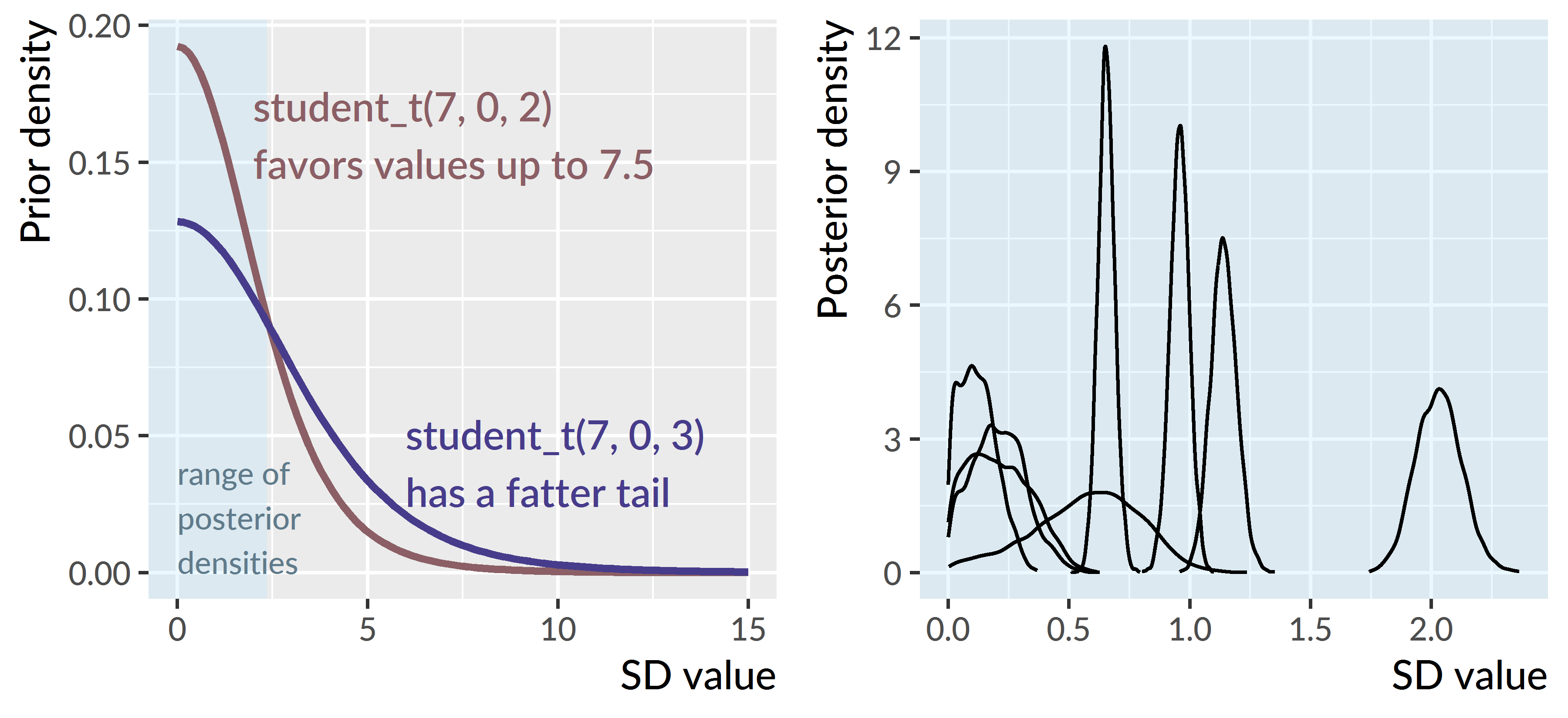
Figure D.1: Prior densities (left) versus posterior densities (right) for the random-effect standard deviations. I changed the prior to be tighter, so that it favor values up to 7.5. This prior still turned out to be very conservative, given that the posterior samples for these values are all less than 3.
Model summary for unfamiliar-initial mispronunciation trials:
summary(mp_unfam, priors = TRUE, prob = .9)
#>  Family: binomial
#>   Links: mu = logit
#> Formula: Target | trials(Trials) ~
#>            (1 + ot1 + ot2 + ot3) * Study +
#>            (1 + ot1 + ot2 + ot3 | ResearchID/Study)
#>    Data: d_u (Number of observations: 11875)
#> Samples: 4 chains, each with iter = 3000; warmup = 1500; thin = 1;
#>          total post-warmup samples = 6000
#>
#> Priors:
#> b ~ normal(0, 1)
#> b_ot1 ~ normal(0, 2)
#> Intercept ~ normal(0, 1)
#> L ~ lkj_corr_cholesky(2)
#> sd ~ student_t(7, 0, 2)
#>
#> Group-Level Effects:
#> ~ResearchID (Number of levels: 193)
#>                    Estimate Est.Error l-90% CI u-90% CI Eff.Sample Rhat
#> sd(Intercept)          0.21      0.11     0.03     0.40         66 1.04
#> sd(ot1)                0.57      0.22     0.16     0.90        111 1.05
#> sd(ot2)                0.21      0.13     0.02     0.44         77 1.05
#> sd(ot3)                0.12      0.08     0.01     0.26        198 1.03
#> cor(Intercept,ot1)    -0.00      0.34    -0.55     0.55        284 1.00
#> cor(Intercept,ot2)     0.04      0.37    -0.59     0.64        432 1.01
#> cor(ot1,ot2)           0.11      0.35    -0.49     0.67        616 1.01
#> cor(Intercept,ot3)    -0.08      0.36    -0.66     0.52        792 1.00
#> cor(ot1,ot3)           0.02      0.35    -0.55     0.60       1213 1.00
#> cor(ot2,ot3)          -0.10      0.36    -0.66     0.53        658 1.00
#>
#> ~ResearchID:Study (Number of levels: 475)
#>                    Estimate Est.Error l-90% CI u-90% CI Eff.Sample Rhat
#> sd(Intercept)          0.96      0.04     0.89     1.02        185 1.01
#> sd(ot1)                2.03      0.09     1.88     2.19        324 1.02
#> sd(ot2)                1.14      0.05     1.05     1.23        388 1.01
#> sd(ot3)                0.65      0.03     0.60     0.71        865 1.00
#> cor(Intercept,ot1)     0.01      0.06    -0.09     0.10        763 1.00
#> cor(Intercept,ot2)     0.10      0.06    -0.00     0.19       1309 1.00
#> cor(ot1,ot2)          -0.12      0.06    -0.22    -0.02        665 1.01
#> cor(Intercept,ot3)     0.01      0.07    -0.10     0.12       2333 1.00
#> cor(ot1,ot3)          -0.16      0.06    -0.27    -0.06       1707 1.00
#> cor(ot2,ot3)          -0.29      0.06    -0.39    -0.19       2053 1.00
#>
#> Population-Level Effects:
#>                     Estimate Est.Error l-90% CI u-90% CI Eff.Sample Rhat
#> Intercept              -0.54      0.08    -0.67    -0.41        704 1.00
#> ot1                     3.36      0.17     3.07     3.63       1520 1.00
#> ot2                    -1.02      0.10    -1.20    -0.85       1360 1.00
#> ot3                     0.39      0.06     0.28     0.49       2244 1.00
#> StudyTimePoint2         0.15      0.11    -0.02     0.33        492 1.00
#> StudyTimePoint3         0.45      0.11     0.27     0.63        712 1.00
#> ot1:StudyTimePoint2    -0.28      0.22    -0.65     0.09       1455 1.00
#> ot1:StudyTimePoint3    -0.29      0.23    -0.67     0.09       1408 1.00
#> ot2:StudyTimePoint2     0.03      0.14    -0.20     0.26       1202 1.00
#> ot2:StudyTimePoint3     0.01      0.14    -0.21     0.24       1232 1.01
#> ot3:StudyTimePoint2    -0.11      0.08    -0.25     0.02       2310 1.00
#> ot3:StudyTimePoint3     0.01      0.09    -0.13     0.15       2622 1.00
#>
#> Samples were drawn using sampling(NUTS). For each parameter, Eff.Sample
#> is a crude measure of effective sample size, and Rhat is the potential
#> scale reduction factor on split chains (at convergence, Rhat = 1).
Model summary for familiar-initial mispronunciation trials:
summary(mp_fam, priors = TRUE, prob = .9)
#>  Family: binomial
#>   Links: mu = logit
#> Formula: Target | trials(Trials) ~
#>            (1 + ot1 + ot2 + ot3) * Study +
#>            (1 + ot1 + ot2 + ot3 | ResearchID/Study)
#>    Data: d_f (Number of observations: 12100)
#> Samples: 4 chains, each with iter = 2000; warmup = 1000; thin = 1;
#>          total post-warmup samples = 4000
#>
#> Priors:
#> b ~ normal(0, 1)
#> b_ot1 ~ normal(0, 2)
#> Intercept ~ normal(0, 1)
#> L ~ lkj_corr_cholesky(2)
#> sd ~ student_t(7, 0, 2)
#>
#> Group-Level Effects:
#> ~ResearchID (Number of levels: 195)
#>                    Estimate Est.Error l-90% CI u-90% CI Eff.Sample Rhat
#> sd(Intercept)          0.44      0.08     0.31     0.55        171 1.04
#> sd(ot1)                0.73      0.24     0.25     1.06         70 1.05
#> sd(ot2)                0.21      0.10     0.04     0.37         97 1.04
#> sd(ot3)                0.08      0.05     0.01     0.18        240 1.02
#> cor(Intercept,ot1)    -0.01      0.25    -0.42     0.39        403 1.01
#> cor(Intercept,ot2)     0.40      0.30    -0.15     0.81        376 1.01
#> cor(ot1,ot2)          -0.29      0.33    -0.74     0.36        252 1.02
#> cor(Intercept,ot3)     0.13      0.35    -0.48     0.66       1555 1.00
#> cor(ot1,ot3)          -0.18      0.35    -0.71     0.45       1159 1.00
#> cor(ot2,ot3)           0.08      0.36    -0.53     0.66       1358 1.00
#>
#> ~ResearchID:Study (Number of levels: 484)
#>                    Estimate Est.Error l-90% CI u-90% CI Eff.Sample Rhat
#> sd(Intercept)          0.84      0.04     0.79     0.91        434 1.01
#> sd(ot1)                1.95      0.10     1.79     2.11        195 1.01
#> sd(ot2)                1.11      0.05     1.04     1.19        727 1.00
#> sd(ot3)                0.62      0.03     0.57     0.66       1578 1.00
#> cor(Intercept,ot1)    -0.05      0.06    -0.16     0.05        678 1.00
#> cor(Intercept,ot2)    -0.02      0.06    -0.12     0.08        544 1.01
#> cor(ot1,ot2)          -0.21      0.06    -0.30    -0.11        705 1.00
#> cor(Intercept,ot3)    -0.06      0.07    -0.16     0.05       1189 1.00
#> cor(ot1,ot3)          -0.05      0.07    -0.16     0.06       1254 1.00
#> cor(ot2,ot3)          -0.49      0.05    -0.57    -0.40       1595 1.00
#>
#> Population-Level Effects:
#>                     Estimate Est.Error l-90% CI u-90% CI Eff.Sample Rhat
#> Intercept               0.76      0.07     0.64     0.88       1660 1.00
#> ot1                    -3.01      0.17    -3.29    -2.74       1502 1.00
#> ot2                     2.00      0.09     1.85     2.15       1286 1.00
#> ot3                    -0.52      0.06    -0.61    -0.42       2008 1.00
#> StudyTimePoint2        -0.23      0.09    -0.39    -0.08       1394 1.00
#> StudyTimePoint3        -0.01      0.09    -0.17     0.14       1651 1.00
#> ot1:StudyTimePoint2     0.56      0.21     0.21     0.92       1489 1.00
#> ot1:StudyTimePoint3     1.30      0.21     0.94     1.64       1508 1.00
#> ot2:StudyTimePoint2    -0.01      0.13    -0.23     0.20       1198 1.00
#> ot2:StudyTimePoint3    -0.26      0.13    -0.48    -0.03       1179 1.00
#> ot3:StudyTimePoint2    -0.11      0.08    -0.24     0.02       2008 1.00
#> ot3:StudyTimePoint3    -0.10      0.08    -0.23     0.03       1939 1.00
#>
#> Samples were drawn using sampling(NUTS). For each parameter, Eff.Sample
#> is a crude measure of effective sample size, and Rhat is the potential
#> scale reduction factor on split chains (at convergence, Rhat = 1).
D.3 Item-response analysis for novel word retention
This is an item-response analysis carried out using a Bayesian mixed-effects logistic regression model. These models were fit in R (vers. 3.5.0; R Core Team, 2018) with the brms package (vers. 2.3.1; Bürkner, 2017). I used weakly informative priors.
The linear model Correct ~ ItemType * c_peak_10 says to estimate the log-odds of answering correctly using on mispronunciations (intercept) using the growth curve peaks (c_peak_10), adjust it for nonwords (ItemType) and for the nonword × peak interaction. The peaks were mean-centered within each type and multiplied by 10 so that the slope represents the effect of change of .1 from the mean peak value. The model includes four random intercepts: general child ability and child × condition ability adjustments (simultaneously requested using 1 | ResearchID/ItemType, i.e., ResearchID levels have ItemType levels nested under / them), plus specific item-level difficulties (1 | Item) and item-pair level difficulties (1 | WordGroup).
d <- readr::read_csv("./data/mp-norming-data.csv.gz")

priors <- c(
  # Population-average intercept
  set_prior(class = "Intercept", "normal(0, 1)"),
  # Population-average slopes
  set_prior(class = "b", "normal(0, 1)"),
  # Standard deviation of the distribution from
  # which random-intercepts are drawn
  set_prior(class = "sd", "student_t(7, 0, 2)"))

m_norm <- brm(
  Correct ~ ItemType * c_peak_10 +
    (1 | ResearchID/ItemType) +
    (1 | WordGroup) +
    (1 | Item),
  prior = priors,
  family = bernoulli,
  chains = 4,
  iter = 2000,
  cores = 4,
  control = list(adapt_delta = .99),
  data = d)

readr::write_rds(m_norm, "./data/mp-norming-m2.rds.gz")
Model summary for retention trials at age 5:
summary(m_norm, priors = TRUE, prob = .9)
#>  Family: bernoulli
#>   Links: mu = logit
#> Formula: Correct ~
#>            ItemType * c_peak_10 +
#>            (1 | ResearchID/ItemType) + (1 | WordGroup) + (1 | Item)
#>    Data: d (Number of observations: 1200)
#> Samples: 4 chains, each with iter = 2000; warmup = 1000; thin = 1;
#>          total post-warmup samples = 4000
#>
#> Priors:
#> b ~ normal(0, 1)
#> Intercept ~ normal(0, 1)
#> sd ~ student_t(7, 0, 2)
#>
#> Group-Level Effects:
#> ~Item (Number of levels: 12)
#>               Estimate Est.Error l-90% CI u-90% CI Eff.Sample Rhat
#> sd(Intercept)     0.67      0.22     0.37     1.08       1468 1.00
#>
#> ~ResearchID (Number of levels: 101)
#>               Estimate Est.Error l-90% CI u-90% CI Eff.Sample Rhat
#> sd(Intercept)     0.34      0.17     0.05     0.62        454 1.01
#>
#> ~ResearchID:ItemType (Number of levels: 200)
#>               Estimate Est.Error l-90% CI u-90% CI Eff.Sample Rhat
#> sd(Intercept)     0.47      0.19     0.11     0.76        419 1.00
#>
#> ~WordGroup (Number of levels: 6)
#>               Estimate Est.Error l-90% CI u-90% CI Eff.Sample Rhat
#> sd(Intercept)     0.46      0.36     0.05     1.11       1152 1.00
#>
#> Population-Level Effects:
#>                           Estimate Est.Error l-90% CI u-90% CI
#> Intercept                     0.57      0.37    -0.03     1.16
#> ItemTypenonword               0.90      0.40     0.22     1.54
#> c_peak_10                    -0.12      0.06    -0.22    -0.02
#> ItemTypenonword:c_peak_10     0.04      0.14    -0.20     0.28
#>                           Eff.Sample Rhat
#> Intercept                       1992 1.00
#> ItemTypenonword                 2180 1.00
#> c_peak_10                       4000 1.00
#> ItemTypenonword:c_peak_10       4000 1.00
#>
#> Samples were drawn using sampling(NUTS). For each parameter, Eff.Sample
#> is a crude measure of effective sample size, and Rhat is the potential
#> scale reduction factor on split chains (at convergence, Rhat = 1).
References
R Core Team. (2018). R: A language and environment for statistical computing. Vienna, Austria: R Foundation for Statistical Computing. Retrieved from https://www.R-project.org/
Bürkner, P.-C. (2017). brms: An R package for Bayesian multilevel models using Stan. Journal of Statistical Software, 80(1), 1–28. doi:10.18637/jss.v080.i01