Chapter 10 Method
Data collection for this experiment occurred during the same longitudinal study as the familiar word recognition experiment of Study 1. Thus, this experiment used the same participants, the same stimulus preparation and style, and the same general experimental procedure as those reported in detail in Chapter 4.
10.1 Mispronunciation task
This experiment is an adaptation of the mispronunciation detection task by White and Morgan (2008) and Law and Edwards (2015). In the experiment, two images are presented onscreen—a familiar object and an unfamiliar object—and the child hears a prompt to view one of the images. In the correct pronunciation (or real word) and mispronunciation conditions, the child hears either the familiar word (e.g., duck) or a one-feature mispronunciation of the first consonant of the target word (guck). These conditions are designed to test whether children associate mispronunciations with novel objects. To encourage fast referent selection, there were also trials in a nonword condition where the label was an unambiguous novel word (e.g., shann presented with images of a cup and a novel-looking bassoon reed). Each nonword was constructed to match the phonotactic probability of one of the mispronunciations. Figure 10.1 shows the screens used in two trials. Importantly, within a block of trials, the child never hears both the correct and mispronounced forms of the same word. A child hearing “duck” then a few trials later hearing “guck” would provide a basis of comparison so that the child can decide that “guck” is probably not “duck”—the design used here avoided this situation and is a change from the design of Law and Edwards (2015).
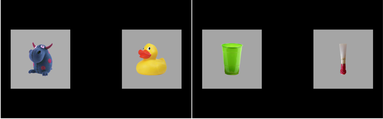
Figure 10.1: Example displays for a trial in which duck is mispronounced as “guck” (left) and a trial in which the nonword shann is presented (right).
In a block of the experiment, there were 12 trials each from the correct production, mispronunciation, and nonword conditions, and children received two blocks of the task. A complete list of the items used in the experiment over the three years of the study is included in Appendix C.
10.2 Visual stimuli
The images used in the experiment consisted of color photographs on gray backgrounds. As in the familiar word recognition experiment, these images were piloted in two preschool classrooms. Piloting confirmed that children consistently used the same label for familiar objects. For the novel objects, the children reported to not know a word for the object, or if they did name the object, they did not consistently use the same word for an object.
10.3 Novel word retention tests
At age 5, following the second block of this task, we tested children’s retention of the labels for the novel objects. They were first tested using an open-set procedure: They were shown each of the images and asked to name it. I will not analyze or report those results, because children seldom named the novel objects using the labels from the task. For example, the rainbow-filled flasks used for sooze (mispronounced shoes) were called science, potions, magic, bottles, among other labels.
Following the open-set naming test, children had a closed-set recognition test. Two of the novel objects were paired. One of the objects was from a mispronunciation trial and the other was from a nonword trial. For example, the toy creature (guck) was paired with the bassoon reed (shann) from the nonword condition. The pairs were yoked, as each nonword was designed to match the phonotactic probability of one of the mispronunciations. During the retention test, children saw two images of the novel objects (say, reed1.jpeg and toy1.jpeg) printed on a letter-size sheet of paper, heard one of novel labels (shann), and had to point to the named object. Figure 10.2 shows an example of what the children saw when tested on guck and shann. In a later trial, the other label (guck) was tested but using different image assets for the objects (toy2.jpeg and reed2.jpeg). In a block of testing, there were 12 trials, 6 for nonwords and 6 for mispronunciations.
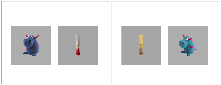
Figure 10.2: Examples of retention trials that tested guck and shann. During the first retention trial (left), children heard one of the unfamiliar words (e.g., guck). The correct response was to point to the toy bull creature because it was the unfamiliar object used on the duck–guck trials. During a later trial that used different image assets (right), children heard the other word (shann). The correct response was to point to the bassoon reed because it was the unfamiliar object used on the shann trials.
10.4 Data screening
Table 10.1 shows the numbers of participants and trials excluded during each of year of the study due to unreliable data. There were more children in the second year than the first year due to a timing error in the initial version of this experiment, leading to the exclusion of 30 participants from the first year.
| Dataset | Year | Children | Blocks | Trials | Percent Missing |
|---|---|---|---|---|---|
| Raw | Age 3 | 177 | 341 | 12245 | 25.4% |
| Age 4 | 181 | 349 | 12600 | 21.4% | |
| Age 5 | 164 | 325 | 11736 | 16.7% | |
| Screened | Age 3 | 162 | 305 | 9062 | 7.9% |
| Age 4 | 170 | 320 | 10031 | 8.1% | |
| Age 5 | 157 | 306 | 10113 | 7.8% | |
| Raw − Screened | Age 3 | 15 | 36 | 3183 | 17.6% |
| Age 4 | 11 | 29 | 2569 | 13.3% | |
| Age 5 | 7 | 19 | 1623 | 8.9% |
After mapping the gaze coordinates onto the onscreen images, I performed data screening following the same set of steps as in Chapter 4. To make data quality judgments, I only considered the window from 0 to 2000 ms after noun onset. Next, I identified a trial as unreliable if at least 50% of the looks were missing during the time window, and I excluded an entire block of trials if it had fewer than 18 reliable trials. As an additional criterion, I excluded participants who failed to provide at least 6 reliable trials per experimental condition.
10.4.1 Classifying trials based on initial fixation location
During preliminary visualization of the age-level growth curves, I observed an increasing preference for the unfamiliar image for the nonword condition—see Figure 10.3. The growth curves showed a typical pattern of a baseline at noun onset followed by a quick change in height as the word unfolded. For the nonword condition, this baseline level moved further from .5 (chance with two images) with each year of the study: Children became more likely to fixate on the novel object at the start of these trials.
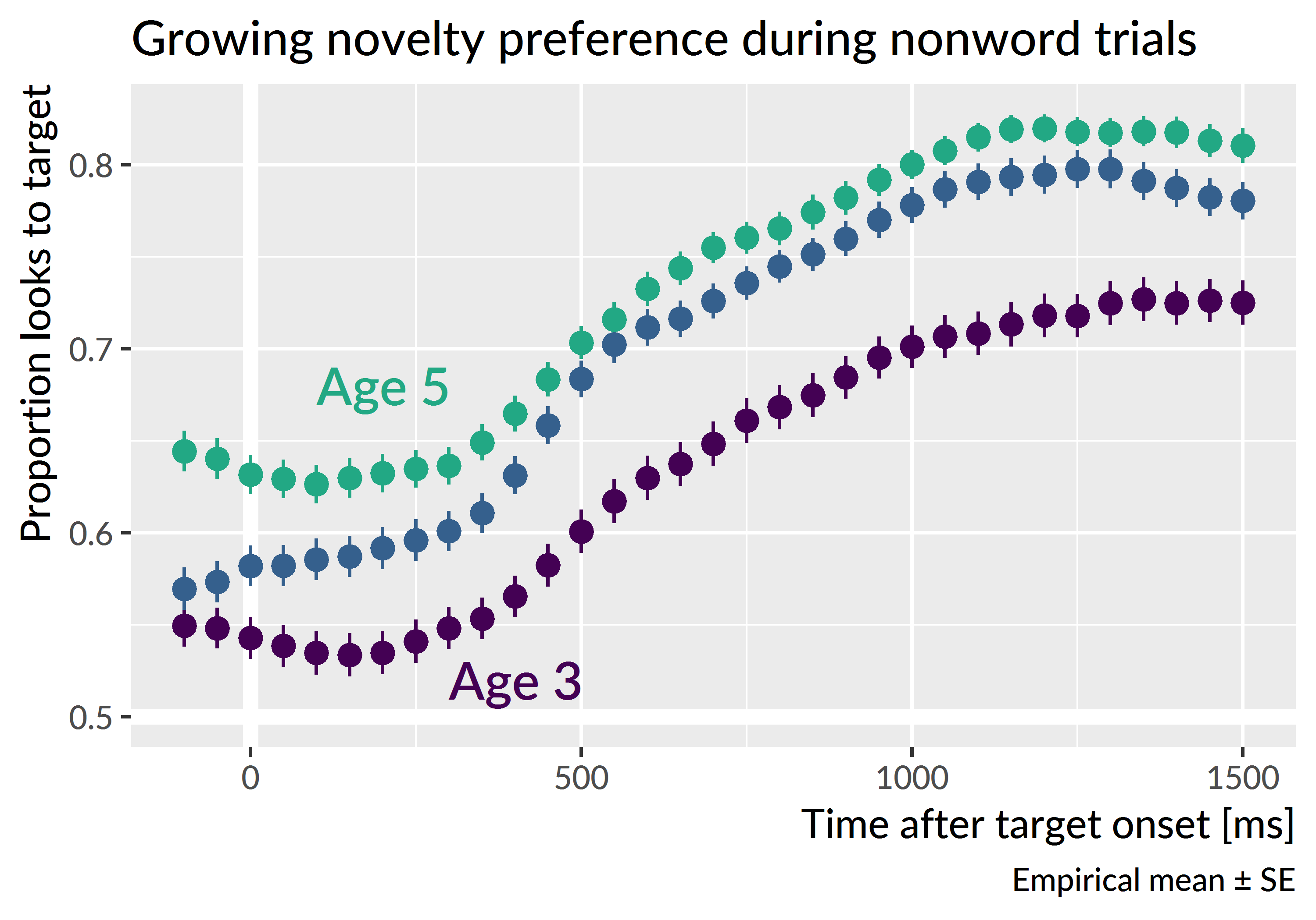
Figure 10.3: Observed average looks to the target on nonword trials. At the onset of the target noun, there is a novelty preference that increases with each year of the study. This novelty preference is the motivation for separating trials based on gaze location at target onset. Points and intervals represent the mean and standard error of children’s empirical growth curves.
Because this was a two-image task, I was able to account for the location of the child’s gaze at the onset of the target noun. For each trial, I counted the number of looks to the familiar object and the unfamiliar object during the first 250 ms after target noun onset (specifically, 0 ≤ time < 250 ms). If the majority of the looks landed on the familiar object, then the trial was a familiar-initial trial. An analogous rule labeled trials as unfamiliar-initial trials. Ties were broken by favoring the earlier fixated image on the assumption that the earlier image better reflected the child’s fixation location at the onset of the target word. For example, a tie might be a trial with 7 frames of looking to the unfamiliar image, followed by 1 frame between the two images, followed by 7 frames to the familiar image. In this case, the unfamiliar image was viewed first, so the trial is classified as unfamiliar-initial. If there were no looks to either image during that window, the trial was not classified for either image and it was excluded.
Table 10.2 shows the counts and percentages of trial classification. About 5% of trials were excluded because the child looked to neither image during the first 250 ms of the noun onset. The table shows how the percentage of unfamiliar-initial trials increased with each year of the study. Accounting for this trend was the rationale for classifying trials based on the initial fixation location.
| Year | Condition | Familiar initial | Unfamiliar initial | Neither/excluded |
|---|---|---|---|---|
| Age 3 | Real word | 1629 (53.7%) | 1250 (41.2%) | 154 (5.10%) |
| Nonword | 1284 (43.8%) | 1453 (49.6%) | 194 (6.60%) | |
| Mispronunciation | 1608 (51.9%) | 1305 (42.1%) | 185 (6.00%) | |
| Age 4 | Real word | 1561 (45.9%) | 1693 (49.8%) | 145 (4.30%) |
| Nonword | 1280 (39.2%) | 1799 (55.2%) | 183 (5.60%) | |
| Mispronunciation | 1686 (50.0%) | 1552 (46.1%) | 132 (3.90%) | |
| Age 5 | Real word | 1718 (50.5%) | 1558 (45.8%) | 125 (3.70%) |
| Nonword | 1172 (35.2%) | 1959 (58.9%) | 194 (5.80%) | |
| Mispronunciation | 1752 (51.7%) | 1487 (43.9%) | 148 (4.40%) |
10.5 Model preparation
To prepare the data for modeling, I downsampled the data into 50-ms (3-frame) bins. I modeled looks from 300 to 1,500 ms after noun onset. Lastly, I aggregated looks by child, year, condition, initial fixation location, and time, and I created orthogonal polynomials to use as time features for the model. Figure 10.4, Figure 10.5, and Figure 10.6 shows the empirical growth curves for each condition following the above-described data screening and preparation steps.
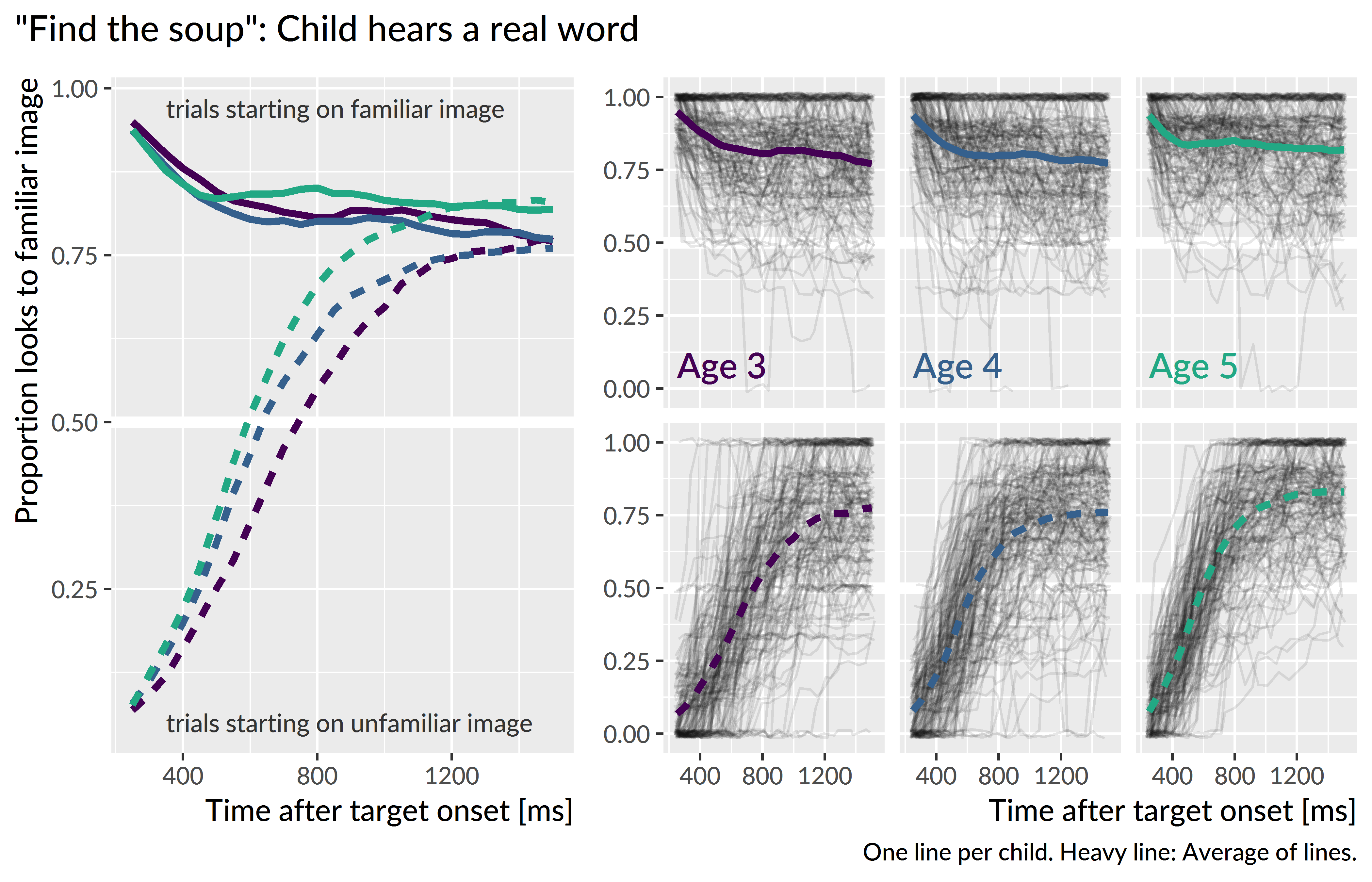
Figure 10.4: Empirical word recognition growth curves for the real words. Each line represents an individual child’s proportion of looks to the target image over time. The heavy lines are the averages of the lines for each year. Only the steep, upward growth curves from unfamiliar-initial trials are analyzed.
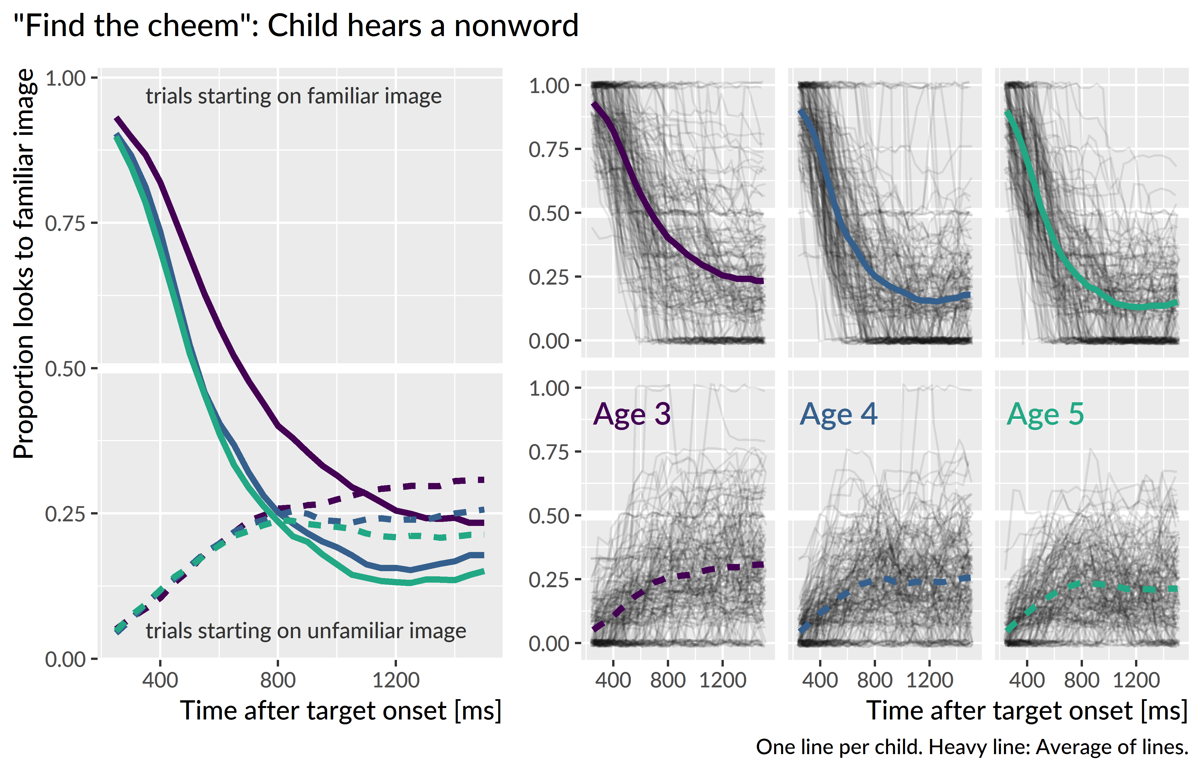
Figure 10.5: Empirical word recognition growth curves for the nonwords. Only the steep, downward growth curves from familiar-initial trials are analyzed.
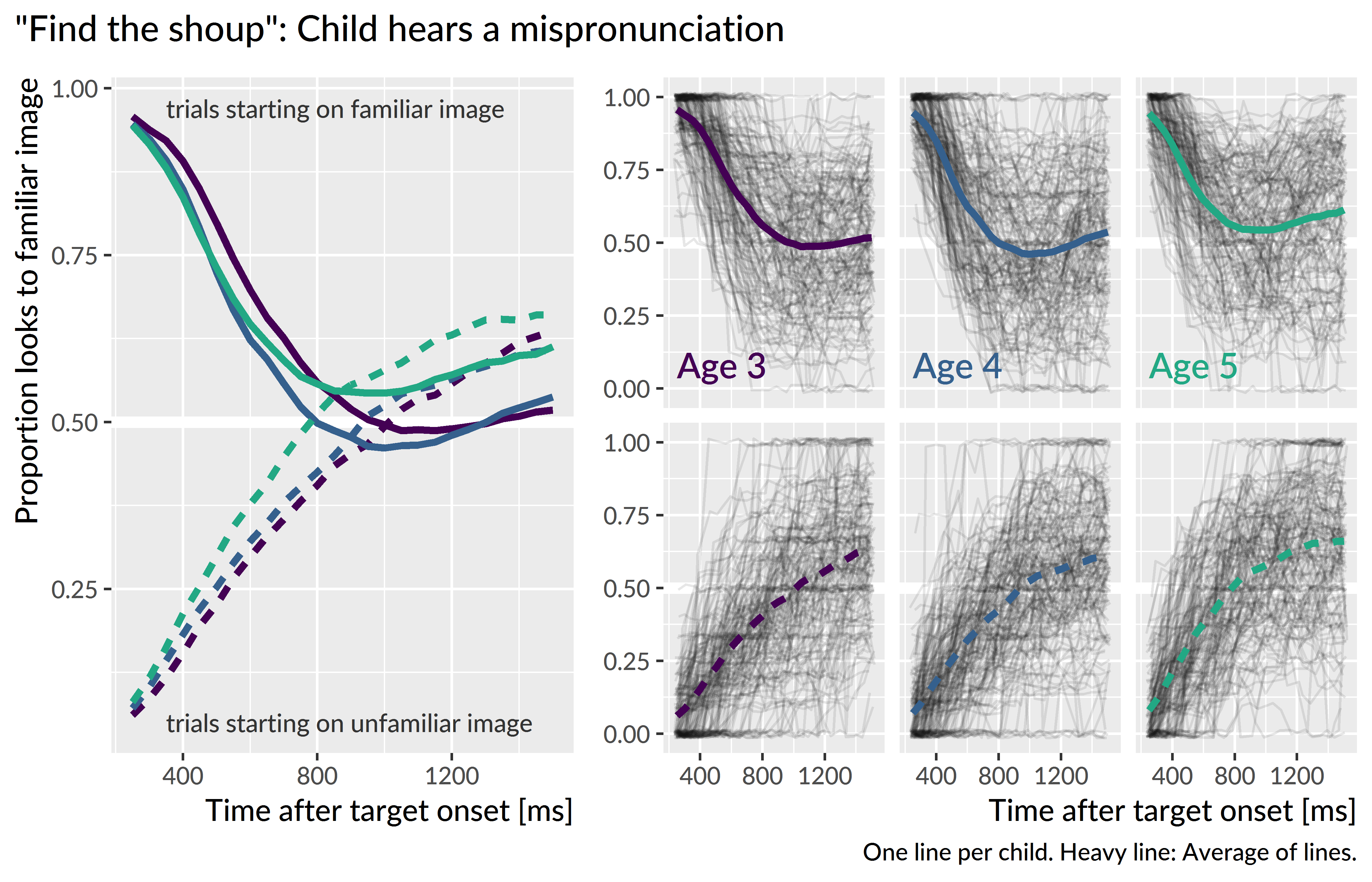
Figure 10.6: Empirical word recognition growth curves for the mispronunciations. Both types of curves are analyzed.
References
White, K. S., & Morgan, J. L. (2008). Sub-segmental detail in early lexical representations. Journal of Memory and Language, 59(1), 114–132. doi:10.1016/j.jml.2008.03.001
Law, F., II, & Edwards, J. R. (2015). Effects of vocabulary size on online lexical processing by preschoolers. Language Learning and Development, 11(4), 331–355. doi:10.1080/15475441.2014.961066