B Computational details for Study 1
B.1 Growth curve analyses
These models were fit in R (vers. 3.4.3; R Core Team, 2018) with the RStanARM package (vers. 2.16.3; Gabry & Goodrich, 2018).
When I computed the orthogonal polynomial features for Time, they were scaled so that the linear feature ranged from −.5 to .5. Under this scaling a unit change in Time1 was equal to change from the start to the end of the analysis window. Table B.1 shows the ranges of the time features.
| Feature | Min | Max | Range |
|---|---|---|---|
| Time1 | −0.50 | 0.50 | 1.00 |
| Time2 | −0.33 | 0.60 | 0.93 |
| Time3 | −0.63 | 0.63 | 1.26 |
| Trial window (ms) | 250 | 1500 | 1250 |
It took approximately 24 hours to run the model on four Monte Carlo sampling chains with 1,000 warm-up iterations and 1,000 sampling iterations. Warm-up iterations are discarded, so the model comprises 4,000 samples from the posterior distribution.
The code used to fit the model with RStanARM is printed below. The variables ot1, ot2, and ot3 are the polynomial time features, ResearchID identifies children, and Study identifies the age/year of the longitudinal project. Mnemonically, ot stands for orthogonal time and the number is the degree of the polynomial. This convention is used by Mirman (2014). Study refers to the timepoint (year) of the larger longitudinal investigation. Conceptually, I use study to mean a data-collection unit, and I think of each wave of testing with their somewhat different tasks and protocols as separate studies. Primary counts the number of looks to the target image at each time bin; Others counts looks to the other three images. cbind(Primary, Others) is used to package both counts together for a logistic regression.
library(rstanarm)

# Run chains on different cores
options(mc.cores = parallel::detectCores())

m <- stan_glmer(
  cbind(Primary, Others) ~
    (ot1 + ot2 + ot3) * Study +
    (ot1 + ot2 + ot3 | ResearchID/Study),
  family = binomial,
  prior = normal(0, 1),
  prior_intercept = normal(0, 5),
  prior_covariance = decov(2, 1, 1),
  control = list(
    adapt_delta = .95,
    max_treedepth = 15),
  data = d_m)

# Save the output
readr::write_rds(m, "./data/stan_aim1_cubic_model.rds.gz")
The code cbind(Primary, Others) ~ (ot1 + ot2 + ot3) * Study fits a cubic growth curve for each age. This code uses R’s formula syntax to regress the looking counts onto an intercept term (implicitly included by default), ot1, ot2, ot3 along with the interactions of the Study variable with the intercept, ot1, ot2, and ot3.
The line (ot1 + ot2 + ot3 | ResearchID/Study) describes the random-effect structure of the model with the / indicating that data from each Study is nested within each ResearchID. Put another way, ... | ResearchID/Study expands into ... | ResearchID and ... | ResearchID:Study. Thus, for each child, we have general ResearchID effects for the intercept, Time1, Time2, and Time3. These child-level effects are further adjusted using Study:ResearchID effects. The effects in each level are allowed to correlate. For example, I would expect that participants with low average looking probabilities (low intercepts) to have flatter growth curves (low Time1 effects), and this relationship would be captured by one of the random-effect correlation terms.
Printing the model object reports the point estimates of the model fixed effects and point-estimate correlation matrices for the random effects.
print(m, digits = 2)
#> stan_glmer
#>  family:       binomial [logit]
#>  formula:      cbind(Primary, Others) ~
#>                  (ot1 + ot2 + ot3) * Study +
#>                  (ot1 + ot2 + ot3 | ResearchID/Study)
#>  observations: 12584
#> ------
#>                     Median MAD_SD
#> (Intercept)         -0.47   0.03
#> ot1                  1.57   0.06
#> ot2                  0.05   0.04
#> ot3                 -0.18   0.03
#> StudyTimePoint2      0.41   0.03
#> StudyTimePoint3      0.70   0.04
#> ot1:StudyTimePoint2  0.56   0.08
#> ot1:StudyTimePoint3  1.10   0.08
#> ot2:StudyTimePoint2 -0.16   0.05
#> ot2:StudyTimePoint3 -0.35   0.05
#> ot3:StudyTimePoint2 -0.12   0.04
#> ot3:StudyTimePoint3 -0.21   0.04
#>
#> Error terms:
#>  Groups           Name        Std.Dev. Corr
#>  Study:ResearchID (Intercept) 0.3054
#>                   ot1         0.6914    0.20
#>                   ot2         0.4367   -0.11  0.02
#>                   ot3         0.2938   -0.11 -0.44 -0.06
#>  ResearchID       (Intercept) 0.2635
#>                   ot1         0.4228    0.78
#>                   ot2         0.1251   -0.75 -0.56
#>                   ot3         0.0576   -0.23 -0.31  0.19
#> Num. levels: Study:ResearchID 484, ResearchID 195
#>
#> Sample avg. posterior predictive distribution of y:
#>          Median MAD_SD
#> mean_PPD 49.86   0.06
#>
#> ------
#> For info on the priors used see help('prior_summary.stanreg').
The model used the following priors:
prior_summary(m)
#> Priors for model 'm'
#> ------
#> Intercept (after predictors centered)
#>  ~ normal(location = 0, scale = 5)
#>
#> Coefficients
#>  ~ normal(location = [0,0,0,...], scale = [1,1,1,...])
#>      **adjusted scale = [3.33,3.33,3.33,...]
#>
#> Covariance
#>  ~ decov(reg. = 2, conc. = 1, shape = 1, scale = 1)
#> ------
#> See help('prior_summary.stanreg') for more details
The priors for the intercept and regression coefficients are wide, weakly informative normal distributions. These distributions are centered at 0, so negative and positive effects are equally likely. The intercept distribution as a standard deviation of 5, and the coefficients have a standard deviation of around 3. On the log-odds scale, 95% looking to target would be 2.94, so effects of this magnitude are easily accommodated by distributions like Normal(0 [mean], 3 [SD]) and Normal(0, 5).
These priors are very conservative, including information about the size of an effect but not its direction. Gelman and Carlin (2014) describe two types of errors that can arise when estimating an effect or model parameter: Type S errors where the sign of the estimated effect is wrong and Type M errors where the magnitude of the estimated effect is wrong. From this perspective, the priors here are uninformative in terms of the sign: Both positive and negative effects are equally likely before seeing the data. Future work on these models should incorporate sign information into the priors: For example, it is a safe bet that the linear time effect will be positive—the curves goes up—so that prior can be adjusted to have a positive, non-zero mean. For this model, I incorporated weak information regarding the magnitude of the effects (an SD of 3 for all effects). On the basis of the estimates here, I employed more informative priors in Study 2 with an SD of 2 for the linear time effect and an SD of 1 for other effects.
For the random-effect part of the model, I used RStanARM’s decov() prior which simultaneously sets a prior on the variances and correlations of the model’s random effect terms. I used the default prior for the variance terms and applied a weakly informative LKJ(2) prior on the random-effect correlations. Figure B.1 shows samples from the prior distribution of two dummy models fit with the default LKJ(1) prior and the weakly informative LKJ(2) prior used here. Under LKJ(2), extreme correlations are less plausible; the prior shifts the probability mass away from the ±1 boundaries towards the center. The motivation for this kind of prior was regularization: I give the model a small amount of information to nudge it away from extreme, degenerate values.
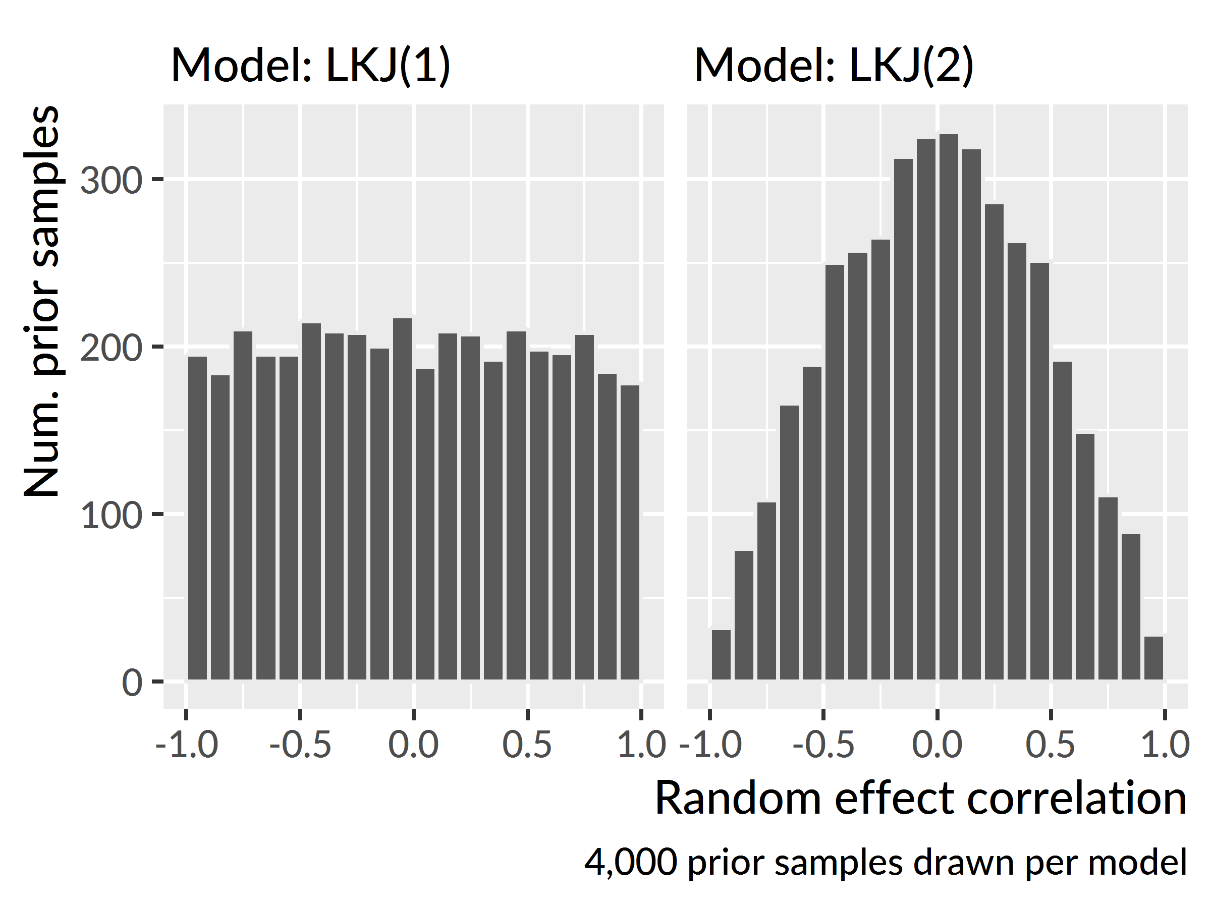
Figure B.1: Samples of correlation effects drawn from LKJ(1) and LKJ(2) priors.
Summary of the familiar word recognition model with diagnostics and 90% uncertainty intervals:
# the last 20 column names are the random effects
ranef_names <- tail(colnames(as_tibble(m)), 20)

summary(
  object = m,
  pars = c("alpha", "beta", ranef_names),
  probs = c(.05, .95),
  digits = 3)
#>
#> Model Info:
#>
#>  function:     stan_glmer
#>  family:       binomial [logit]
#>  formula:      cbind(Primary, Others) ~
#.                  (ot1 + ot2 + ot3) * Study +
#.                  (ot1 + ot2 + ot3 | ResearchID/Study)
#>  algorithm:    sampling
#>  priors:       see help('prior_summary')
#>  sample:       4000 (posterior sample size)
#>  observations: 12584
#>  groups:       Study:ResearchID (484), ResearchID (195)
#>
#> Estimates:
#>                                          mean     sd     5%    95%
#> (Intercept)                            -0.469  0.032 -0.523 -0.419
#> ot1                                     1.575  0.066  1.465  1.682
#> ot2                                     0.048  0.038 -0.014  0.110
#> ot3                                    -0.175  0.026 -0.218 -0.130
#> StudyTimePoint2                         0.410  0.035  0.355  0.468
#> StudyTimePoint3                         0.697  0.035  0.641  0.757
#> ot1:StudyTimePoint2                     0.565  0.079  0.437  0.695
#> ot1:StudyTimePoint3                     1.099  0.080  0.968  1.233
#> ot2:StudyTimePoint2                    -0.157  0.052 -0.242 -0.073
#> ot2:StudyTimePoint3                    -0.354  0.053 -0.443 -0.267
#> ot3:StudyTimePoint2                    -0.121  0.036 -0.181 -0.061
#> ot3:StudyTimePoint3                    -0.213  0.036 -0.275 -0.155
#> Sigma[Study:ResearchID:(Intercept),(Intercept)]
#>                                         0.093  0.008  0.081  0.107
#> Sigma[Study:ResearchID:ot1,(Intercept)] 0.042  0.013  0.022  0.064
#> Sigma[Study:ResearchID:ot2,(Intercept)]
#>                                        -0.015  0.008 -0.029 -0.001
#> Sigma[Study:ResearchID:ot3,(Intercept)]
#>                                        -0.010  0.005 -0.019 -0.001
#> Sigma[Study:ResearchID:ot1,ot1]         0.478  0.043  0.411  0.551
#> Sigma[Study:ResearchID:ot2,ot1]         0.006  0.019 -0.026  0.036
#> Sigma[Study:ResearchID:ot3,ot1]        -0.089  0.013 -0.111 -0.069
#> Sigma[Study:ResearchID:ot2,ot2]         0.191  0.015  0.166  0.217
#> Sigma[Study:ResearchID:ot3,ot2]        -0.007  0.008 -0.019  0.005
#> Sigma[Study:ResearchID:ot3,ot3]         0.086  0.008  0.074  0.099
#> Sigma[ResearchID:(Intercept),(Intercept)]
#>                                         0.069  0.012  0.051  0.090
#> Sigma[ResearchID:ot1,(Intercept)]       0.087  0.018  0.060  0.117
#> Sigma[ResearchID:ot2,(Intercept)]      -0.025  0.009 -0.040 -0.011
#> Sigma[ResearchID:ot3,(Intercept)]      -0.004  0.004 -0.011  0.003
#> Sigma[ResearchID:ot1,ot1]               0.179  0.043  0.113  0.252
#> Sigma[ResearchID:ot2,ot1]              -0.030  0.015 -0.056 -0.006
#> Sigma[ResearchID:ot3,ot1]              -0.008  0.008 -0.022  0.004
#> Sigma[ResearchID:ot2,ot2]               0.016  0.008  0.005  0.030
#> Sigma[ResearchID:ot3,ot2]               0.001  0.002 -0.002  0.006
#> Sigma[ResearchID:ot3,ot3]               0.003  0.002  0.001  0.008
#>
#> Diagnostics:
#>                                                 mcse  Rhat  n_eff
#> (Intercept)                                     0.001 1.005 1086
#> ot1                                             0.002 1.004  857
#> ot2                                             0.001 1.006  842
#> ot3                                             0.001 1.002 1156
#> StudyTimePoint2                                 0.001 1.007 1034
#> StudyTimePoint3                                 0.001 1.006  959
#> ot1:StudyTimePoint2                             0.003 1.014  674
#> ot1:StudyTimePoint3                             0.003 1.005  934
#> ot2:StudyTimePoint2                             0.002 1.003  836
#> ot2:StudyTimePoint3                             0.002 1.006  762
#> ot3:StudyTimePoint2                             0.001 1.003 1183
#> ot3:StudyTimePoint3                             0.001 1.001 1390
#> Sigma[Study:ResearchID:(Intercept),(Intercept)] 0.000 1.002 1093
#> Sigma[Study:ResearchID:ot1,(Intercept)]         0.001 1.009  475
#> Sigma[Study:ResearchID:ot2,(Intercept)]         0.000 1.023  323
#> Sigma[Study:ResearchID:ot3,(Intercept)]         0.000 1.003  792
#> Sigma[Study:ResearchID:ot1,ot1]                 0.002 1.003  547
#> Sigma[Study:ResearchID:ot2,ot1]                 0.001 1.013  277
#> Sigma[Study:ResearchID:ot3,ot1]                 0.000 1.005  806
#> Sigma[Study:ResearchID:ot2,ot2]                 0.001 1.010  665
#> Sigma[Study:ResearchID:ot3,ot2]                 0.000 1.001 1131
#> Sigma[Study:ResearchID:ot3,ot3]                 0.000 1.004 1220
#> Sigma[ResearchID:(Intercept),(Intercept)]       0.000 1.004  913
#> Sigma[ResearchID:ot1,(Intercept)]               0.001 1.008  636
#> Sigma[ResearchID:ot2,(Intercept)]               0.001 1.026  307
#> Sigma[ResearchID:ot3,(Intercept)]               0.000 1.006  711
#> Sigma[ResearchID:ot1,ot1]                       0.003 1.010  261
#> Sigma[ResearchID:ot2,ot1]                       0.001 1.021  242
#> Sigma[ResearchID:ot3,ot1]                       0.000 1.006  331
#> Sigma[ResearchID:ot2,ot2]                       0.000 1.037  257
#> Sigma[ResearchID:ot3,ot2]                       0.000 1.009  439
#> Sigma[ResearchID:ot3,ot3]                       0.000 1.007  340
#>
#> For each parameter, mcse is Monte Carlo standard error, n_eff is a
#> crude measure of effective sample size, and Rhat is the potential
#> scale reduction factor on split chains (at convergence Rhat=1).
B.1.1 Convergence diagnostics for Bayesian models
For the Bayesian models estimated in Study 1 and Study 2, I assessed model convergence by checking software warnings and checking sampling diagnostics. Stan programs emit warnings when the Hamiltonian Monte Carlo sampler runs into problems like divergent transitions or a low Bayesian Fraction of Missing Information statistic. When I encountered these warnings, I handled them by adjusting the sampling controls, as documented in <http://mc-stan.org/misc/warnings.html>, or incorporating more information into the model’s priors. In the above model, for example, the adapt_delta and max_treedepth controls were increased to help the model more carefully explore the posterior distribution.
rstan::check_hmc_diagnostics(m$stanfit)
#>
#> Divergences:
#> 3 of 4000 iterations ended with a divergence (0.075%).
#> Try increasing 'adapt_delta' to remove the divergences.
#>
#> Tree depth:
#> 0 of 4000 iterations saturated the maximum tree depth of 15.
#>
#> Energy:
#> E-BFMI indicated no pathological behavior.
Additionally, I also checked for convergence by using Markov Chain Monte Carlo diagnostics. The models consisted of four sampling chains which explore the posterior distribution from random starting locations. The split \(\hat{R}\) (“R-hat”) diagnostic checks how well the sampling chains mix together (Gelman et al., 2014, p. 285; Stan Development Team, 2017, p. 371). If the chains are stuck in their own neighborhoods of the parameter space, then the values sampled in each chain will not mix very well. The split designation means that each chain is first split in half so that the also diagnostic checks for within-chain mixing. At convergence \(\hat{R}\) equals 1, so a rule of thumb is that \(\hat{R}\) should be less than 1.1 (e.g., Gelman et al., 2014, p. 285). In the bayesplot package (Gabry & Mahr, 2018), we use the convention that values below 1.05 are good and values above 1.05 but below than 1.1 are okay.
The other diagnostic I monitored was the number of effective samples. If we think of a sampling chain as exploring a parameter space, then the samples form a random walk with each step being a movement from an earlier location. This situation raises the risk of autocorrelation where neighboring sampling steps within a chain are correlated with each other. The number of effective samples (“n eff.”) diagnostic estimates the number of posterior samples, taking into account sampling autocorrelation (Gelman et al., 2014, p. 285; Stan Development Team, 2017, p. 373). The square root of this number is used to calculate Monte Carlo standard error statistics (e.g., Gelman et al., 2014, p. 267), so I think of the number of effective samples as the amount of precision available for a parameter estimate. Interpreting this statistic depends on the quantity being estimated and the amount of precision desired. As a rule of thumb, Gelman et al. (2014) mentions 10 effective samples per chain as a baseline for diagnosing non-convergence: “Having an effective sample size of 10 per sequence should typically correspond to stability of all the simulated sequences. For some purposes, more precision will be desired, and then a higher effective sample size threshold can be used. [p. 287]”
B.2 Generalized additive models
To model the looks to the competitor images, I used generalized additive (mixed) models. The models were fit in R (vers. 3.4.3) using the mgcv R package (vers. 1.8.23; Wood, 2017) with support from tools in the itsadug R package (vers. 2.3; van Rij et al., 2017).
I will briefly walk through the code used to fit one of these models in order to articulate the modeling decisions at play. I first convert the categorical variables into the right types, so that the model can fit difference smooths.
# Create a Study dummy variabe with Age 4 as the reference level
phon_d$S <- factor(
  phon_d$Study,
  levels = c("TimePoint2", "TimePoint1", "TimePoint3"))

# Convert the ResearchID into a factor
phon_d$R <- as.factor(phon_d$ResearchID)

# Convert the Study factor (phon_d$S) into an ordered factor.
# This step is needed for the ti model estimate difference smooths.
phon_d$S2 <- as.ordered(phon_d$S)
contrasts(phon_d$S2) <- "contr.treatment"
contrasts(phon_d$S2)
I fit the generalized additive model with the code below. The outcome elog is the empirical log-odds of looking to the phonological competitor relative to the unrelated word.
library(mgcv)

phon_gam <- bam(
  elog ~ S2 +
    s(Time) + s(Time, by = S2) +
    s(Time, R, bs = "fs", m = 1, k = 5),
  data = phon_d)

# Save the output
readr::write_rds(phon_gam, "./data/aim1-phon-random-smooths.rds.gz")
There is just one parametric term: S2. The term computes the average effect of each study with Age 4 serving as the reference condition (and as the model intercept).
Next come the smooth terms. s(Time) fits the shape of Time for the reference condition (Age 4). s(Time, by = S2) fits the difference smooths for Age 3 versus Age 4 and Age 5 versus Age 4. s(Time, R, bs = "fs", m = 1, k = 5) fits a smooth for each participant (R). bs = "fs" means that the model should use a factor smooth (fs) basis (bs)—that is, a “random effect” smooth for each participant. m = 1 changes the smoothness penalty so that the random effects are pulled towards the group average; Winter and Wieling (2016) and Baayen, Rij, Cat, and Wood (2016) suggest using this option. k = 5 means to use 5 knots (k) for the basis function. The other smooths use the default number of knots (10). I used fewer knots for the by-child smooths because of limited data. As a result, these smooths capture by-child variation by making coarse adjustments to study-level growth curves.
Summary of the phonological model:
m_p <- readr::read_rds("./data/aim1-phon-random-smooths.rds.gz")
summary(m_p)
#>
#> Family: gaussian
#> Link function: identity
#>
#> Formula:
#> elog ~ S2 + s(Time) + s(Time, by = S2) + s(Time, R, bs = "fs",
#>     m = 1, k = 5)
#>
#> Parametric coefficients:
#>               Estimate Std. Error t value Pr(>|t|)
#> (Intercept)   0.159200   0.048807   3.262  0.00111 **
#> S2TimePoint1 -0.002641   0.013840  -0.191  0.84864
#> S2TimePoint3  0.151073   0.013601  11.107  < 2e-16 ***
#> ---
#> Signif. codes:  0 '***' 0.001 '**' 0.01 '*' 0.05 '.' 0.1 ' ' 1
#>
#> Approximate significance of smooth terms:
#>                          edf  Ref.df     F  p-value
#> s(Time)                7.277   8.165 10.61 3.51e-15 ***
#> s(Time):S2TimePoint1   5.478   6.590 17.10  < 2e-16 ***
#> s(Time):S2TimePoint3   1.001   1.002 17.86 2.37e-05 ***
#> s(Time,R)            852.928 974.000 12.97  < 2e-16 ***
#> ---
#> Signif. codes:  0 '***' 0.001 '**' 0.01 '*' 0.05 '.' 0.1 ' ' 1
#>
#> R-sq.(adj) =  0.311   Deviance explained = 33.1%
#> fREML =  41726  Scale est. = 0.8629    n = 30008
Summary of the semantic model:
m_s <- readr::read_rds("./data/aim1-semy-random-smooths.rds.gz")
summary(m_s)
#>
#> Family: gaussian
#> Link function: identity
#>
#> Formula:
#> elog ~ S2 + s(Time) + s(Time, by = S2) + s(Time, R, bs = "fs",
#>     m = 1, k = 5)
#>
#> Parametric coefficients:
#>              Estimate Std. Error t value Pr(>|t|)
#> (Intercept)   0.43878    0.04907   8.943  < 2e-16 ***
#> S2TimePoint1 -0.13985    0.01352 -10.345  < 2e-16 ***
#> S2TimePoint3  0.06486    0.01329   4.881 1.06e-06 ***
#> ---
#> Signif. codes:  0 '***' 0.001 '**' 0.01 '*' 0.05 '.' 0.1 ' ' 1
#>
#> Approximate significance of smooth terms:
#>                          edf  Ref.df      F  p-value
#> s(Time)                7.038   7.988 11.018 1.16e-15 ***
#> s(Time):S2TimePoint1   1.001   1.001  0.387 0.534636
#> s(Time):S2TimePoint3   3.739   4.623  4.909 0.000323 ***
#> s(Time,R)            867.572 974.000 15.750  < 2e-16 ***
#> ---
#> Signif. codes:  0 '***' 0.001 '**' 0.01 '*' 0.05 '.' 0.1 ' ' 1
#>
#> R-sq.(adj) =  0.379   Deviance explained = 39.7%
#> fREML =  42860  Scale est. = 0.85001   n = 30976
References
R Core Team. (2018). R: A language and environment for statistical computing. Vienna, Austria: R Foundation for Statistical Computing. Retrieved from https://www.R-project.org/
Gabry, J., & Goodrich, B. (2018). RStanARM: Bayesian applied regression modeling via Stan. Retrieved from https://CRAN.R-project.org/package=rstanarm
Mirman, D. (2014). Growth curve analysis and visualization using R. Boca Raton, FL: CRC Press/Taylor & Francis Group.
Gelman, A., & Carlin, J. (2014). Beyond power calculations: Assessing Type S (sign) and Type M (magnitude) errors. Perspectives on Psychological Science, 9(6), 641–651. doi:10.1177/1745691614551642
Gelman, A., Carlin, J. B., Stern, H. S., Dunson, D. B., Vehtari, A., & Rubin, D. B. (2014). Bayesian data analysis (3rd ed.). Boca Raton, FL: CRC Press/Taylor & Francis Group.
Stan Development Team. (2017). Stan modeling language: User’s guide and reference manual.
Gabry, J., & Mahr, T. (2018). bayesplot: Plotting for Bayesian models. Retrieved from https://CRAN.R-project.org/package=bayesplot
Wood, S. N. (2017). Generalized additive models: An introduction with R (2nd ed.). Boca Raton, FL: CRC Press/Taylor & Francis Group.
van Rij, J., Wieling, M., Baayen, R. H., & van Rijn, H. (2017). itsadug: Interpreting time series and autocorrelated data using GAMMs.
Winter, B., & Wieling, M. (2016). How to analyze linguistic change using mixed models, growth curve analysis and generalized additive modeling. Journal of Language Evolution, 1(1), 7–18. doi:10.1093/jole/lzv003
Baayen, R. H., Rij, J. van, Cat, C. de, & Wood, S. N. (2016). Autocorrelated errors in experimental data in the language sciences: Some solutions offered by generalized additive mixed models. Retrieved from http://arxiv.org/abs/1601.02043