Added variable plots (partial regression plots)

Here’s what “added variable” plots are about.

• Let m = y ~ x1 + ... be the full regression model
• Let m_y1 = y ~ ... (all of the predictors except x1)
• Let m_x1 = x1 ~ ... (regress x1 on those same predictors)
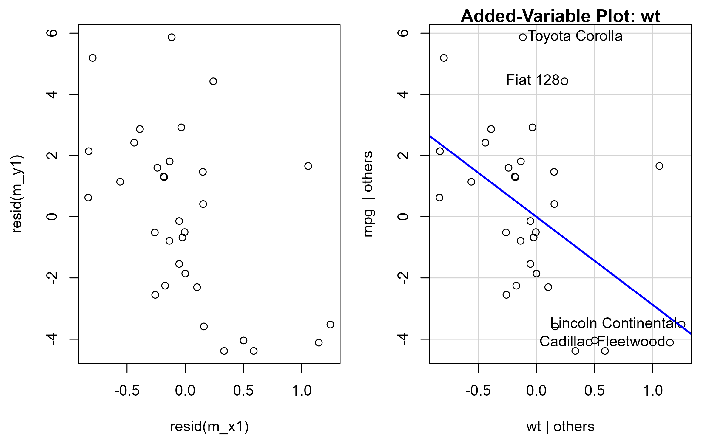
• Let m_partial = resid(m_y1) ~ resid(m_x1)
• The plot of resid(m_x1) versus resid(m_y1) is the added variable plot. It shows “X1 | others)” and “y | others”
• Residuals in the final m_partial model will be same as residuals from full model m
• Coefficient of x1 in final m_partial model will be same as coefficient from full model m.

AV plots by hand and by car::avPlot()

par(mar = c(4, 4, 1, 1))

m <- lm(mpg ~ wt + hp + am, mtcars)
m_y1 <- lm(mpg ~ hp + am, mtcars)
m_x1 <- lm(wt ~ hp + am, mtcars)
m_partial <- lm(resid(m_y1) ~ resid(m_x1))

library(patchwork)
p1 <- wrap_elements(
  full = ~ plot(resid(m_x1), resid(m_y1))
) 
p2 <- wrap_elements(
  full = ~ car::avPlot(m, "wt")
)

p1 + p2

center

all.equal(residuals(m_partial), residuals(m))
#> [1] TRUE

coef(m)["wt"]
#>        wt 
#> -2.878575
coef(m_partial)[2]
#> resid(m_x1) 
#>   -2.878575

What about interactions?