Standardizing gamma distributions via scaling

A gamma times a positive non-zero constant is still a gamma. Paul and I used this fact to standardize results from different models onto a single “z” scale. Here’s a made-up example.

Simulate some gamma-distributed data.

library(patchwork)
set.seed(20211122)
par(mar = c(4, 4, 1, 1))

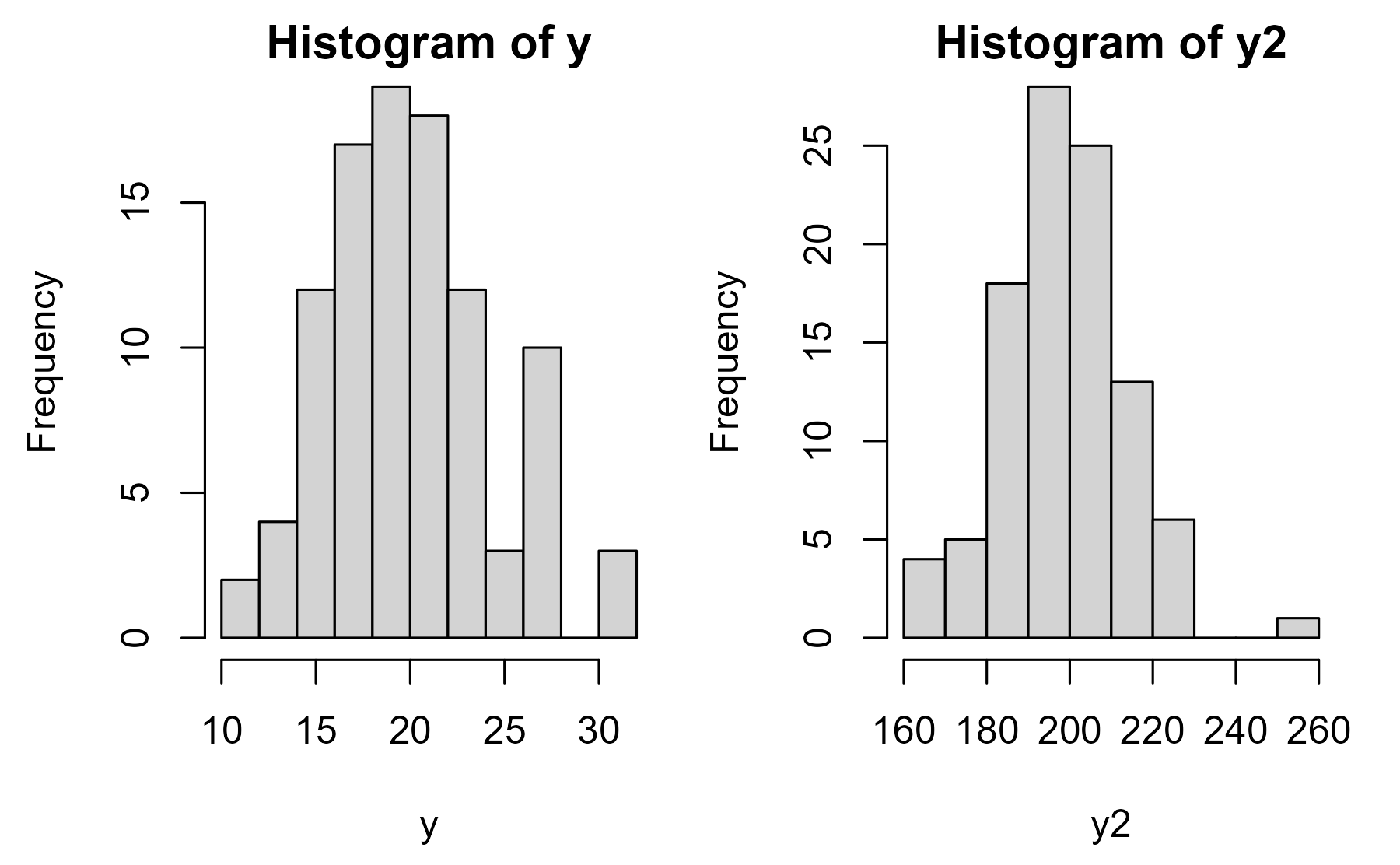
y <- rgamma(n = 100, shape = 20)
y2 <- rgamma(n = 100, shape = 200)
wrap_elements(full = ~ hist(y)) + 
  wrap_elements(full = ~ hist(y2))

center

Fit a GLM

get_shape <- function(model) { 
  1 / summary(model)[["dispersion"]]
}

m <- glm(y ~ 1, Gamma(link = "identity"))
m2 <- glm(y2 ~ 1, Gamma(link = "identity"))

get_shape(m)
#> [1] 21.09197
get_shape(m2)
#> [1] 178.6259

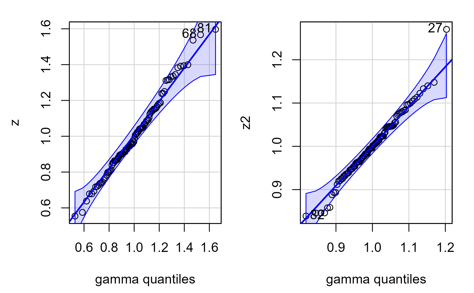
The two z values have similar scales.

par(mar = c(4, 4, 1, 1))
r <- residuals(m)
r2 <- residuals(m2)

z <- y / fitted(m)
z2 <- y2 / fitted(m2)

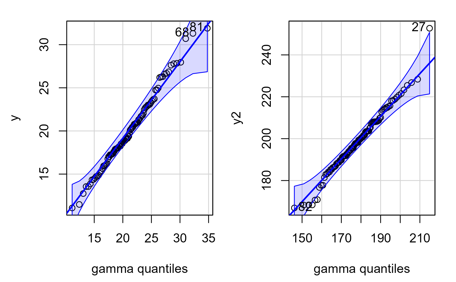
p1 <- wrap_elements(
  full = ~ car::qqPlot(y, distribution = "gamma", shape = get_shape(m))
)
p2 <- wrap_elements(
  full = ~ car::qqPlot(y2, distribution = "gamma", shape = get_shape(m2))
)
p1 + p2

center

p3 <- wrap_elements(
  full = ~ car::qqPlot(
    z, 
    distribution = "gamma", 
    shape = get_shape(m), 
    scale = 1 / get_shape(m))
)  
p4 <- wrap_elements(
  full = ~ car::qqPlot(
    z2, 
    distribution = "gamma", 
    shape = get_shape(m2), 
    scale = 1 / get_shape(m2))
)
p3 + p4

center