Ridgelines in bayesplot 1.5.0
At the end of March, Jonah Gabry and I released bayesplot 1.5.0. The major additions to the package were visualizations using ridgelines and a new plot for PIT diagnostics from LOO validation. I don’t know what that LOO PIT thing is yet, so I’ll talk about how ridgelines have been incorporated into bayesplot instead.

Ridgelines display the distributions of some variables—think of a series of bell curves—but allow the curves to vary in height or overlap each other. Several curves packed together look like a mountain ridge (hence the name). The canonical example of this visualization are the cold, austere lines from the cover of Joy Division’s Unknown Pleasures.
In this post, I briefly describe where ridgelines appear in the package now. At the end of the post, I show a more involved example of fitting a model and plotting results from it.
Behind the scenes of mcmc_areas()
I’m going to start with a less obvious use of ridgelines. mcmc_areas()
visualizes the posterior distribution of model parameters. It helps us see where
the peak values are, and occasionally, whether there is more than one peak. By
default, it will plot the complete range of the distribution, shade the
middle 50% of the distribution, and draw a line at the median.
For this release, I rewrote the function so that it uses the ggridges package. I had noticed that the shapes it produced had different areas. Here’s an example of how the plots have changed.
Update: A reproducibility puzzle
Hello from February 2021. I decided to rebuild this blog post. But at
this time, the bayesplot had moved onto version 1.8.0 so the content of
the post would not be describing the behavior of 1.5.0. This situation
created a little reproducibility puzzle. Full
reproducibility—traveling back in time and using the versions of
ggplot2, ggridges, etc.—would be too difficult, and frankly, not worth
the hassle. But it is important for the next plot to reproduce how the
area definition in bayesplot for mcmc_areas() changed from v1.4.0 to
v1.5.0—and while we are at it—from v1.5.0 to now.
After some troubleshooting and experimenting, I came up with the following plan.
- Augment the library paths (
.libPaths()) to include a temporary folder, install bayesplot v1.5.0 in it, andlibrary()the package. This will give me bayesplot v1.5.0 for the rest of the post. - In a separate R session (via
callr::r()), do the same thing—temporarily install v1.4.0—and create the plot. Here we usewithr::with_temp_libpaths()to automate the temporary library-path manipulation. - In a separate R session, create the plot using my regular library
paths (
old_lib_pathsin the code below).
# 2021-02-12: This section was overhauled so that
# this post could temporarily reinstall bayesplot 1.5.0
# so the plots in the post are accurate
library(ggplot2)

# Set a temporary library folder for the rest of the post. It
# will house bayesplot 1.5.0 so this post is reproducible
old_lib_paths <- .libPaths()
temp_lib_paths <- c(tempdir(), .libPaths())
.libPaths(temp_lib_paths)

remotes::install_github(
  "stan-dev/bayesplot",
  ref = "v1.5.0",
  quiet = TRUE,
  upgrade = "never"
)

library(bayesplot)
#> This is bayesplot version 1.5.0
#> - Plotting theme set to bayesplot::theme_default()
#> - Online documentation at mc-stan.org/bayesplot
example_data <- example_mcmc_draws()

p_1.5.0 <- mcmc_areas(example_data, c("beta[1]", "beta[2]")) +
  ggtitle(paste0("Version ", packageVersion("bayesplot"))) +
  theme_default()

plot_with_v1.4.0 <- function(data) {
  # Temporarily install the previous version of bayesplot and
  # make an mcmc_areas() plot.
  withr::with_temp_libpaths({
    remotes::install_github(
      "stan-dev/bayesplot",
      ref = "v1.4.0",
      quiet = TRUE,
      upgrade = "never"
    )
    library(ggplot2)
    library(bayesplot)

    p <- mcmc_areas(data, pars = c("beta[1]", "beta[2]")) +
      ggtitle(paste0("Version ", packageVersion("bayesplot"))) +
      theme_default()
  })
  p
}

plot_with_dev <- function(data) {
  library(ggplot2)
  library(bayesplot)

  p <- mcmc_areas(
    data,
    pars = c("beta[1]", "beta[2]")
  ) +
    ggtitle(paste0("Version ", packageVersion("bayesplot"))) +
    theme_default()
  p
}

p_1.4.0 <- callr::r(plot_with_v1.4.0, list(data = example_data))

p_current <- callr::r(
  plot_with_dev,
  list(data = example_data),
  libpath = old_lib_paths
)
Back to the original post
# Show the three together
cowplot::plot_grid(p_1.4.0, p_1.5.0, p_current, nrow = 1)
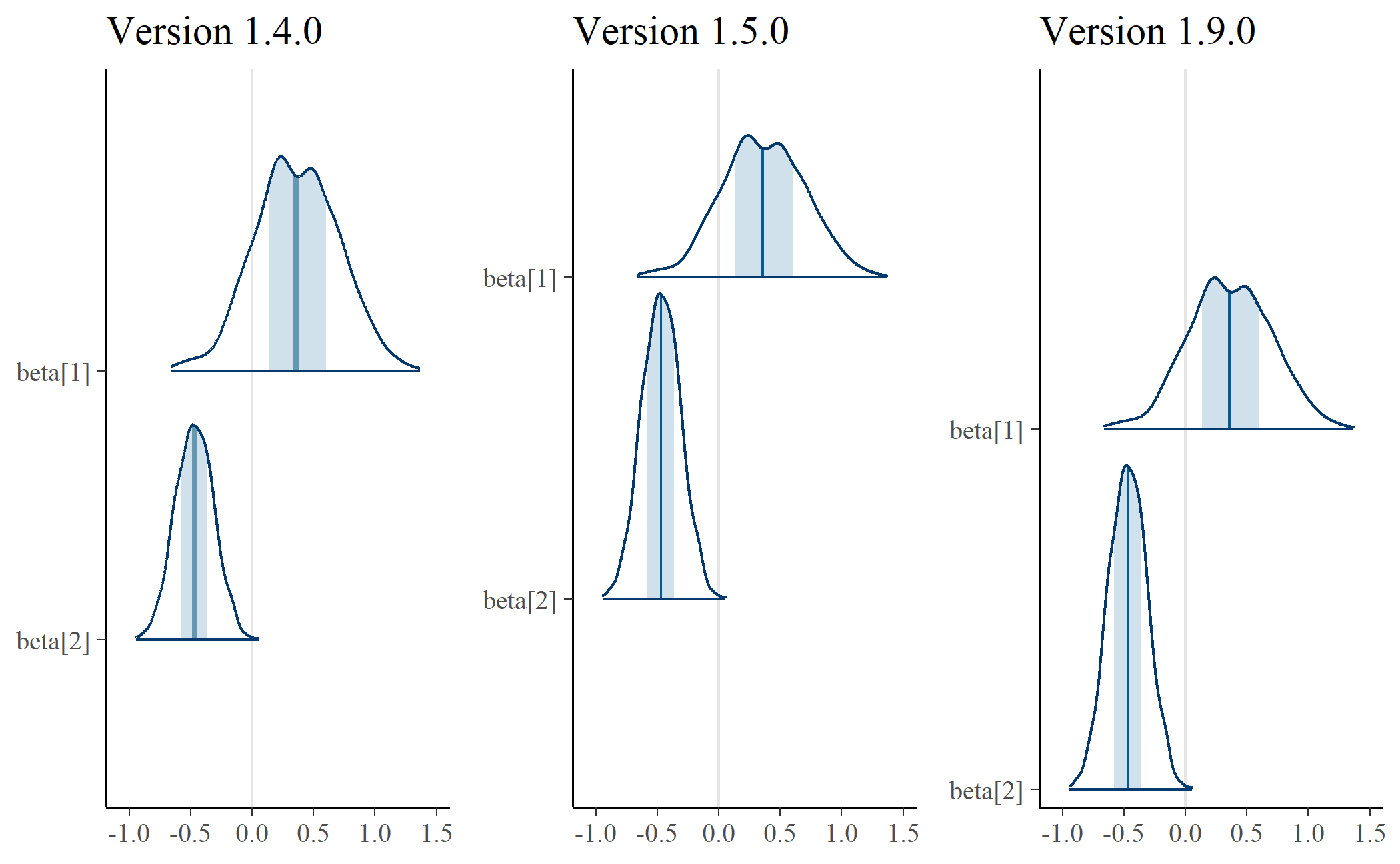
In the plot on the left, the shapes have different areas. Eyeballing it, it
looks like beta[2] would fit inside beta[1]. Area is width times height.
These shapes have different widths because they cover different values—that
makes sense. Therefore, the problem is the height—namely, the fact that the
shapes have the same height. To make the areas more similar, we adjust the
heights, and that’s what’s happening in the plot in the center. The distribution
for beta[2] is concentrated to a more narrow range, and that feature manifests
in that shape’s much higher peak.
Three plots in one
This plot is built using the ggridges packages which handles drawing the shapes at different heights. It took a bit of trickery, however, to do the annotation for the shaded 50% interval and the median. Here is a high-level overview of what’s happening.
mcmc_areas_data() tidies the MCMC samples into a dataframe suitable for
plotting. It computes the density of the parameter values, and it returns the
densities over three intervals: 1) an outer interval, 2) an inner interval to
be shaded, and 3) a narrow “point” interval.
library(dplyr, warn.conflicts = FALSE)

d <- example_data %>%
  mcmc_areas_data(c("beta[1]", "beta[2]")) %>%
  mutate(
    interval = factor(interval, c("outer", "inner", "point"))
  )
d
#> # A tibble: 4,238 × 5
#>    parameter interval interval_width     x density
#>    <fct>     <fct>             <dbl> <dbl>   <dbl>
#>  1 beta[1]   inner               0.5 0.136   0.986
#>  2 beta[1]   inner               0.5 0.137   0.988
#>  3 beta[1]   inner               0.5 0.137   0.989
#>  4 beta[1]   inner               0.5 0.138   0.990
#>  5 beta[1]   inner               0.5 0.138   0.991
#>  6 beta[1]   inner               0.5 0.139   0.992
#>  7 beta[1]   inner               0.5 0.139   0.993
#>  8 beta[1]   inner               0.5 0.139   0.994
#>  9 beta[1]   inner               0.5 0.140   0.995
#> 10 beta[1]   inner               0.5 0.140   0.997
#> # … with 4,228 more rows
Internally, mcmc_areas() uses ggridges::geom_density_ridges() to draw
three different ridgeline plots.
# Separate the full range so it can be drawn on each facet.
full_range <- d %>%
  filter(interval == "outer") %>%
  select(-interval)

p_base <- ggplot(d) +
  aes(x = x, y = parameter, fill = interval, height = density) +
  # For reference include the full-range.
  # `stat = "identity"` means that ggridges should not scale the heights
  ggridges::geom_density_ridges(
    stat = "identity",
    data = full_range,
    color = "grey80",
    size = 1,
    fill = NA
  ) +
  ggridges::geom_density_ridges(stat = "identity") +
  scale_fill_brewer(type = "seq") +
  guides(fill = "none")

p_base +
  facet_wrap("interval")
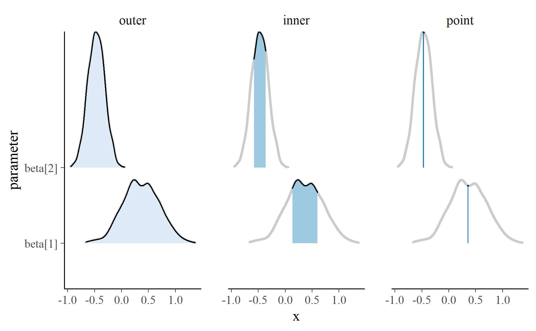
These intervals are layered to achieve the desired look.
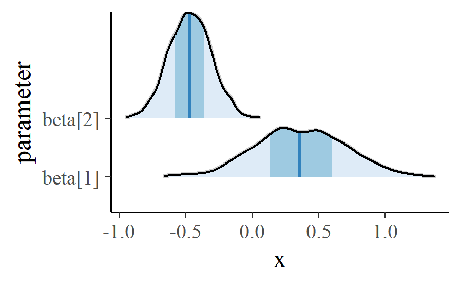
There’s a bit more fussing to the actual function. For example, the width of the intervals and whether a point is calculated are options that have to be handled. The tips of the topmost peaks are not cut off in those plots as well. But that’s the basic idea.
Overlapping ridgelines for related parameters
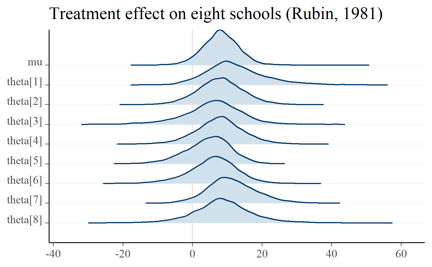
Plots with the classic, overlapping Unknown Pleasures look are supported by
mcmc_areas_ridges(). I like these plots for hierarchical models where the
parameters represent similar units. In fact, part of the reason Jonah approached
me about contributing to bayesplot was a proof-of-concept demo
I wrote to visualize hierarchical effects using ridgeline plots, back when they
were popularly called “joyplots”.
Below is the eight schools example where there is a treatment effect for each school (thetas) and an overall average effect (mu).
m <- shinystan::eight_schools@posterior_sample

mcmc_areas_ridges(m, pars = "mu", regex_pars = "theta") +
  ggtitle("Treatment effect on eight schools (Rubin, 1981)")
If we really want to go for the Unknown Pleasures look, we can manually plot the densities in a white-on-black theme. Most of the work here is padding zero values onto the ridgelines so that they all have the same width.
d <- m %>%
  mcmc_areas_ridges_data(pars = "mu", regex_pars = "theta") %>%
  filter(interval == "outer")

zeroes <- d %>%
  # Get range of each parameter
  group_by(parameter) %>%
  summarise(pmin = min(x), pmax = max(x)) %>%
  mutate(
    min = min(pmin),
    max = max(pmax),
    # On each row, make a data-frame of zeroes from absolute minimum
    # value to this parameter's minimum value
    lower_df = purrr::map2(
      min,
      pmin,
      ~ data.frame(x = seq(.x, .y, length.out = 20), density = 0)
    ),
    # Make a dataframe of zeroes from each parameter's max to the
    # overall max
    upper_df = purrr::map2(
      pmax,
      max,
      ~ data.frame(x = seq(.x, .y, length.out = 20), density = 0)
    ),
    # Gather the zeroes together
    df = purrr::map2(lower_df, upper_df, bind_rows)
  ) %>%
  select(parameter, df) %>%
  tidyr::unnest(df)

ggplot(bind_rows(d, zeroes)) +
  aes(x = x, y = parameter, height = density) +
  ggridges::geom_density_ridges(
    stat = "identity",
    fill = NA,
    color = "grey70",
    scale = 5
  ) +
  theme_void() +
  theme(
    plot.background = element_rect(fill = "black"),
    plot.margin = unit(c(.25, .25, .25, .25), units = "npc"),
    axis.ticks = element_blank()
  )

Densities of different sampling chains
Finally, ridgelines appear in by-chain diagnostics using mcmc_dens_chains().
mcmc_dens_chains(m, pars = c("theta[1]", "theta[2]", "theta[3]"))
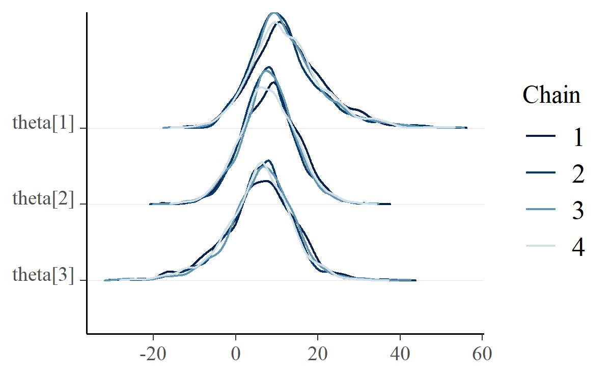
There really isn’t much interesting to say about this plot, except that it follows Mike DeCrescenzo’s early example of using ridgelines on Bayesian models.
An example of fitting and plotting a model
The cake dataset in lme4 reports the angle of breakage of chocolate cakes
for 3 different recipes at 6 temperatures tested 15 times each (3 × 6 × 15 = 270
observations). The data are shown below, ignoring temperature details:
set.seed(20180405)
cake <- lme4::cake

theme_set(theme_grey())

ggplot(cake) +
  # aes(x = temp, y = angle, color = recipe) +
  aes(x = replicate, y = angle, color = recipe) +
  geom_text(aes(label = recipe), position = position_jitter(.15), size = 3) +
  stat_summary(color = "grey10", size = .4) +
  guides(color = FALSE, label = FALSE) +
  labs(
    x = "Replicate",
    y = "Angle of breakage",
    caption = "Letters: Recipe. Points: Replicate Mean ± SE"
  )
#> No summary function supplied, defaulting to `mean_se()`
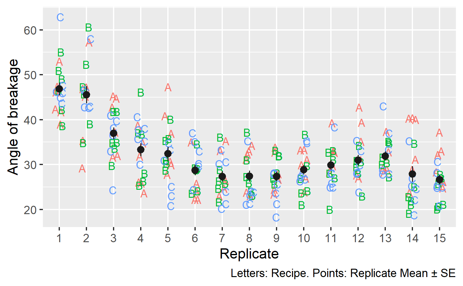
It looks like the first few replications showed larger breakage angles compared to later ones. From a modeling perspective, we would want to capture variation due to replication. There could be variation due to recipe × replication effects, so we will model the data at that level of detail.
# Update 2020-02-12: Fit the model in a separate R session because rstanarm
# currently errors because the version of bayesplot is too old for this post
fit_model <- function(data) {
  library(rstanarm)
  m <- stan_glmer(
    angle ~ recipe * temp + (1 | recipe:replicate),
    family = gaussian(),
    data = data,
    prior = normal(0, 1, autoscale = TRUE),
    seed = 20180405
  )
  as.array(m)
}

m <- callr::r(
  fit_model,
  list(data = cake),
  libpath = old_lib_paths
)
This models predicts the breakage angle using an average recipe, temperature, and recipe × temperate effects and adjusting the prediction for each recipe × replication.
Below, we use mcmc_areas_ridges() to plot the distributions of replication
effects for recipe A. The plotting functions in bayesplot take a set of MCMC
samples from a model. We can extract the samples using as.matrix(). We can
narrow the parameters to be plotted by naming them individually with pars or
by selecting all the parameters that match a regular expression pattern with
regex_pars.
# Revert to the bayesplot default theme
theme_set(bayesplot::theme_default())

mcmc_areas_ridges(m, regex_pars = c("recipe:replicate:A"))
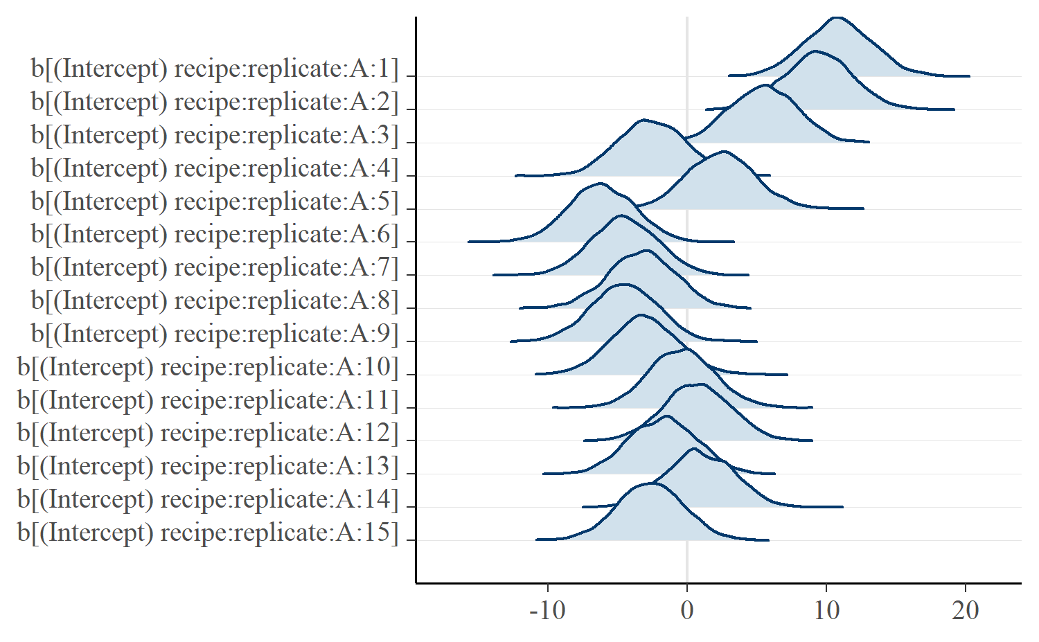
The effects describe deviations from the recipe average. A faint line is drawn at x = 0 represents the average value. Ridges to the left of the line are below average and those to the right are above average. We can see that the model captured how the first three replications had particular high breakage angles.
Last knitted on 2022-05-27. Source code on GitHub.1
-
.session_info
#> ─ Session info ───────────────────────────────────────────────────────────────
#>  setting      value
#>  version      R version 4.2.0 (2022-04-22 ucrt)
#>  os           Windows 10 x64 (build 22000)
#>  system       x86_64, mingw32
#>  ui           RTerm
#>  language     (EN)
#>  collate      English_United States.utf8
#>  ctype        English_United States.utf8
#>  tz           America/Chicago
#>  date         2022-05-27
#>  pandoc       NA
#>  stan (rstan) 2.21.0
#>
#> ─ Packages ───────────────────────────────────────────────────────────────────
#>  ! package      * version  date (UTC) lib source
#>    assertthat     0.2.1    2019-03-21 [2] CRAN (R 4.2.0)
#>    base64enc      0.1-3    2015-07-28 [2] CRAN (R 4.2.0)
#>    bayesplot    * 1.5.0    2022-05-27 [1] Github (stan-dev/bayesplot@e7b1934)
#>    boot           1.3-28   2021-05-03 [3] CRAN (R 4.2.0)
#>    cachem         1.0.6    2021-08-19 [2] CRAN (R 4.2.0)
#>    callr          3.7.0    2021-04-20 [2] CRAN (R 4.2.0)
#>    cli            3.3.0    2022-04-25 [2] CRAN (R 4.2.0)
#>    codetools      0.2-18   2020-11-04 [3] CRAN (R 4.2.0)
#>    colorspace     2.0-3    2022-02-21 [2] CRAN (R 4.2.0)
#>    colourpicker   1.1.1    2021-10-04 [2] CRAN (R 4.2.0)
#>    cowplot        1.1.1    2020-12-30 [2] CRAN (R 4.2.0)
#>    crayon         1.5.1    2022-03-26 [2] CRAN (R 4.2.0)
#>    crosstalk      1.2.0    2021-11-04 [2] CRAN (R 4.2.0)
#>    curl           4.3.2    2021-06-23 [2] CRAN (R 4.2.0)
#>    DBI            1.1.2    2021-12-20 [2] CRAN (R 4.2.0)
#>    digest         0.6.29   2021-12-01 [2] CRAN (R 4.2.0)
#>  R downlit        0.4.0    <NA>       [2] <NA>
#>    dplyr        * 1.0.9    2022-04-28 [2] CRAN (R 4.2.0)
#>    DT             0.23     2022-05-10 [2] CRAN (R 4.2.0)
#>    dygraphs       1.1.1.6  2018-07-11 [2] CRAN (R 4.2.0)
#>    ellipsis       0.3.2    2021-04-29 [2] CRAN (R 4.2.0)
#>    evaluate       0.15     2022-02-18 [2] CRAN (R 4.2.0)
#>    fansi          1.0.3    2022-03-24 [2] CRAN (R 4.2.0)
#>    farver         2.1.0    2021-02-28 [2] CRAN (R 4.2.0)
#>    fastmap        1.1.0    2021-01-25 [2] CRAN (R 4.2.0)
#>    generics       0.1.2    2022-01-31 [2] CRAN (R 4.2.0)
#>    ggplot2      * 3.3.6    2022-05-03 [2] CRAN (R 4.2.0)
#>    ggridges       0.5.3    2021-01-08 [2] CRAN (R 4.2.0)
#>    git2r          0.30.1   2022-03-16 [2] CRAN (R 4.2.0)
#>    glue           1.6.2    2022-02-24 [2] CRAN (R 4.2.0)
#>    gridExtra      2.3      2017-09-09 [2] CRAN (R 4.2.0)
#>    gtable         0.3.0    2019-03-25 [2] CRAN (R 4.2.0)
#>    gtools         3.9.2.1  2022-05-23 [2] CRAN (R 4.2.0)
#>    here           1.0.1    2020-12-13 [2] CRAN (R 4.2.0)
#>    highr          0.9      2021-04-16 [2] CRAN (R 4.2.0)
#>    htmltools      0.5.2    2021-08-25 [2] CRAN (R 4.2.0)
#>    htmlwidgets    1.5.4    2021-09-08 [2] CRAN (R 4.2.0)
#>    httpuv         1.6.5    2022-01-05 [2] CRAN (R 4.2.0)
#>    igraph         1.3.1    2022-04-20 [2] CRAN (R 4.2.0)
#>    inline         0.3.19   2021-05-31 [2] CRAN (R 4.2.0)
#>    knitr        * 1.39     2022-04-26 [2] CRAN (R 4.2.0)
#>    labeling       0.4.2    2020-10-20 [2] CRAN (R 4.2.0)
#>    later          1.3.0    2021-08-18 [2] CRAN (R 4.2.0)
#>    lattice        0.20-45  2021-09-22 [3] CRAN (R 4.2.0)
#>    lifecycle      1.0.1    2021-09-24 [2] CRAN (R 4.2.0)
#>    lme4           1.1-29   2022-04-07 [2] CRAN (R 4.2.0)
#>    loo            2.5.1    2022-03-24 [2] CRAN (R 4.2.0)
#>    magrittr       2.0.3    2022-03-30 [2] CRAN (R 4.2.0)
#>    markdown       1.1      2019-08-07 [2] CRAN (R 4.2.0)
#>    MASS           7.3-56   2022-03-23 [3] CRAN (R 4.2.0)
#>    Matrix         1.4-1    2022-03-23 [3] CRAN (R 4.2.0)
#>    matrixStats    0.62.0   2022-04-19 [2] CRAN (R 4.2.0)
#>    memoise        2.0.1    2021-11-26 [2] CRAN (R 4.2.0)
#>    mime           0.12     2021-09-28 [2] CRAN (R 4.2.0)
#>    miniUI         0.1.1.1  2018-05-18 [2] CRAN (R 4.2.0)
#>    minqa          1.2.4    2014-10-09 [2] CRAN (R 4.2.0)
#>    munsell        0.5.0    2018-06-12 [2] CRAN (R 4.2.0)
#>    nlme           3.1-157  2022-03-25 [3] CRAN (R 4.2.0)
#>    nloptr         2.0.2    2022-05-19 [2] CRAN (R 4.2.0)
#>    pillar         1.7.0    2022-02-01 [2] CRAN (R 4.2.0)
#>    pkgbuild       1.3.1    2021-12-20 [2] CRAN (R 4.2.0)
#>    pkgconfig      2.0.3    2019-09-22 [2] CRAN (R 4.2.0)
#>    plyr           1.8.7    2022-03-24 [2] CRAN (R 4.2.0)
#>    prettyunits    1.1.1    2020-01-24 [2] CRAN (R 4.2.0)
#>    processx       3.5.3    2022-03-25 [2] CRAN (R 4.2.0)
#>    promises       1.2.0.1  2021-02-11 [2] CRAN (R 4.2.0)
#>    ps             1.7.0    2022-04-23 [2] CRAN (R 4.2.0)
#>    purrr          0.3.4    2020-04-17 [2] CRAN (R 4.2.0)
#>    R6             2.5.1    2021-08-19 [2] CRAN (R 4.2.0)
#>    ragg           1.2.2    2022-02-21 [2] CRAN (R 4.2.0)
#>    RColorBrewer   1.1-3    2022-04-03 [2] CRAN (R 4.2.0)
#>    Rcpp           1.0.8.3  2022-03-17 [2] CRAN (R 4.2.0)
#>  D RcppParallel   5.1.5    2022-01-05 [2] CRAN (R 4.2.0)
#>    remotes        2.4.2    2021-11-30 [2] CRAN (R 4.2.0)
#>    reshape2       1.4.4    2020-04-09 [2] CRAN (R 4.2.0)
#>    rlang          1.0.2    2022-03-04 [2] CRAN (R 4.2.0)
#>    rprojroot      2.0.3    2022-04-02 [2] CRAN (R 4.2.0)
#>    rstan          2.21.5   2022-04-11 [2] CRAN (R 4.2.0)
#>    rstudioapi     0.13     2020-11-12 [2] CRAN (R 4.2.0)
#>    scales         1.2.0    2022-04-13 [2] CRAN (R 4.2.0)
#>    sessioninfo    1.2.2    2021-12-06 [2] CRAN (R 4.2.0)
#>    shiny          1.7.1    2021-10-02 [2] CRAN (R 4.2.0)
#>    shinyjs        2.1.0    2021-12-23 [2] CRAN (R 4.2.0)
#>    shinystan      2.6.0    2022-03-03 [2] CRAN (R 4.2.0)
#>    shinythemes    1.2.0    2021-01-25 [2] CRAN (R 4.2.0)
#>    StanHeaders    2.21.0-7 2020-12-17 [2] CRAN (R 4.2.0)
#>    stringi        1.7.6    2021-11-29 [2] CRAN (R 4.2.0)
#>    stringr        1.4.0    2019-02-10 [2] CRAN (R 4.2.0)
#>    systemfonts    1.0.4    2022-02-11 [2] CRAN (R 4.2.0)
#>    textshaping    0.3.6    2021-10-13 [2] CRAN (R 4.2.0)
#>    threejs        0.3.3    2020-01-21 [2] CRAN (R 4.2.0)
#>    tibble         3.1.7    2022-05-03 [2] CRAN (R 4.2.0)
#>    tidyr          1.2.0    2022-02-01 [2] CRAN (R 4.2.0)
#>    tidyselect     1.1.2    2022-02-21 [2] CRAN (R 4.2.0)
#>    utf8           1.2.2    2021-07-24 [2] CRAN (R 4.2.0)
#>    vctrs          0.4.1    2022-04-13 [2] CRAN (R 4.2.0)
#>    withr          2.5.0    2022-03-03 [2] CRAN (R 4.2.0)
#>    xfun           0.31     2022-05-10 [2] CRAN (R 4.2.0)
#>    xtable         1.8-4    2019-04-21 [2] CRAN (R 4.2.0)
#>    xts            0.12.1   2020-09-09 [2] CRAN (R 4.2.0)
#>    yaml           2.3.5    2022-02-21 [2] CRAN (R 4.2.0)
#>    zoo            1.8-10   2022-04-15 [2] CRAN (R 4.2.0)
#>
#>  [1] C:/Users/Tristan/AppData/Local/Temp/Rtmp86uQFe
#>  [2] C:/Users/Tristan/AppData/Local/R/win-library/4.2
#>  [3] C:/Program Files/R/R-4.2.0/library
#>
#>  D ── DLL MD5 mismatch, broken installation.
#>  R ── Package was removed from disk.
#>
#> ──────────────────────────────────────────────────────────────────────────────

Leave a comment