Manually computing spline predictions from a GAMLSS model
My goal is write down some reusable code for how to get spline predictions for unobserved x values by hand from a GAMLSS model.
Problem
Here are 98 random points from a subrange of the intelligibility dataset.
library(tidyverse)
#> Warning: package 'tibble' was built under R version 4.5.2
#> Warning: package 'tidyr' was built under R version 4.5.2
#> Warning: package 'readr' was built under R version 4.5.2
#> Warning: package 'purrr' was built under R version 4.5.2
#> Warning: package 'dplyr' was built under R version 4.5.2
#> Warning: package 'stringr' was built under R version 4.5.2
#> Warning: package 'lubridate' was built under R version 4.5.2
#> ── Attaching core tidyverse packages ──────────────────────── tidyverse 2.0.0 ──
#> ✔ dplyr     1.2.0     ✔ readr     2.2.0
#> ✔ forcats   1.0.1     ✔ stringr   1.6.0
#> ✔ ggplot2   4.0.2     ✔ tibble    3.3.1
#> ✔ lubridate 1.9.5     ✔ tidyr     1.3.2
#> ✔ purrr     1.2.1
#> ── Conflicts ────────────────────────────────────────── tidyverse_conflicts() ──
#> ✖ dplyr::filter() masks stats::filter()
#> ✖ dplyr::lag()    masks stats::lag()
#> ℹ Use the conflicted package (<http://conflicted.r-lib.org/>) to force all conflicts to become errors
suppressMessages(library(gamlss))
#> Warning: package 'nlme' was built under R version 4.5.3
select <- dplyr::select

data_intel <- tibble::tribble(
   ~id, ~age_months, ~mean_intelligibility,
    1L,          44,                  0.74,
    2L,          49,                 0.779,
    3L,          56,                 0.686,
    4L,          51,                 0.675,
    5L,          42,                 0.785,
    6L,          42,                 0.708,
    7L,          38,                 0.557,
    8L,          44,                 0.756,
    9L,          56,                  0.64,
   10L,          50,                 0.767,
   11L,          48,                 0.858,
   12L,          53,                  0.94,
   13L,          49,                 0.673,
   14L,          56,                 0.928,
   15L,          54,                 0.827,
   16L,          51,                 0.868,
   17L,          53,                 0.784,
   18L,          50,                 0.908,
   19L,          37,                 0.458,
   20L,          37,                 0.184,
   21L,          51,                 0.688,
   22L,          53,                 0.753,
   23L,          43,                 0.802,
   24L,          47,                 0.841,
   25L,          45,                 0.523,
   26L,          37,                 0.288,
   27L,          42,                 0.672,
   28L,          50,                 0.777,
   29L,          54,                 0.749,
   30L,          53,                 0.901,
   31L,          55,                 0.806,
   32L,          45,                 0.646,
   33L,          45,                 0.689,
   34L,          45,                 0.806,
   35L,          46,                 0.859,
   36L,          36,                 0.557,
   37L,          38,                 0.606,
   38L,          50,                 0.804,
   39L,          44,                 0.853,
   40L,          51,                 0.747,
   41L,          37,                 0.659,
   42L,          48,                 0.883,
   43L,          45,                 0.798,
   44L,          39,                 0.483,
   45L,          59,                 0.976,
   46L,          58,                 0.786,
   48L,          48,                 0.775,
   49L,          47,                 0.896,
   50L,          38,                 0.921,
   51L,          41,                 0.686,
   53L,          54,                  0.72,
   54L,          51,                 0.965,
   55L,          44,                 0.777,
   56L,          42,                  0.53,
   57L,          36,                 0.707,
   58L,          60,                 0.908,
   59L,          37,                 0.566,
   60L,          51,                 0.598,
   61L,          58,                 0.938,
   62L,          54,                 0.925,
   63L,          47,                 0.757,
   64L,          42,                  0.63,
   65L,          45,                 0.764,
   66L,          59,                  0.85,
   67L,          47,                 0.786,
   68L,          38,                 0.781,
   69L,          44,                 0.929,
   70L,          36,                 0.356,
   71L,          55,                 0.802,
   72L,          54,                 0.864,
   73L,          43,                 0.864,
   74L,          49,                 0.848,
   75L,          38,                 0.574,
   76L,          53,                 0.916,
   77L,          41,                  0.85,
   78L,          59,                 0.851,
   79L,          46,                 0.444,
   80L,          55,                 0.778,
   81L,          54,                 0.931,
   82L,          50,                  0.32,
   83L,          58,                 0.855,
   84L,          39,                  0.64,
   85L,          50,                 0.727,
   86L,          50,                 0.857,
   87L,          39,                 0.731,
   88L,          46,                 0.624,
   89L,          53,                 0.951,
   90L,          46,                 0.873,
   91L,          47,                 0.897,
   92L,          46,                 0.748,
   93L,          59,                 0.936,
   94L,          50,                 0.881,
   95L,          43,                 0.815,
   96L,          44,                 0.768,
   97L,          43,                 0.789,
   98L,          50,                 0.728,
   99L,          38,                 0.794,
  100L,          44,                 0.509
)
data_intel <- data_intel %>%
  arrange(age_months)
But note that we are missing data from three ages (x values).
ggplot(data_intel) +
  aes(x = age_months, y = mean_intelligibility) +
  geom_point() +
  geom_vline(xintercept = c(40, 52, 57), linetype = "dashed") +
  scale_x_continuous(breaks = c(36, 48, 60))
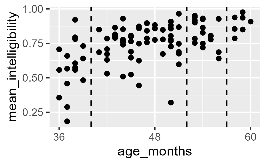
Intelligibility data but there are no observations at 40, 52, and 57 months
Here is how we would fit a beta-regression model as we did in the growth curve paper.
fit_beta_gamlss <- function(data, mu_df = 3, sigma_df = 2) {
  BE <- gamlss.dist::BE
  gamlss.control <- gamlss::gamlss.control
  ns <- splines::ns

  model <- wisclabmisc::mem_gamlss(
    mean_intelligibility ~ ns(age_months, df = mu_df),
    sigma.formula = ~ ns(age_months, df = sigma_df),
    family = BE(),
    data = data,
    control = gamlss.control(trace = FALSE)
  )

  model$.user$mu_df <- mu_df
  model$.user$sigma_df <- sigma_df

  model$.user$mu_basis <- ns(data$age_months, mu_df)
  model$.user$sigma_basis <- ns(data$age_months, sigma_df)

  model
}

model <- fit_beta_gamlss(data_intel, mu_df = 3, sigma_df = 2)
Then we can get centiles pretty easily for the existing x values. But note the three gaps on the percentile line.
centiles <- data_intel %>%
  select(age_months) %>%
  wisclabmisc::predict_centiles(model)

ggplot(data_intel) +
  aes(x = age_months, y = mean_intelligibility) +
  geom_point() +
  geom_point(
    aes(y = c10),
    data = centiles,
    color = "skyblue3",
    size = 10,
    shape = "-"
  ) +
  scale_x_continuous(breaks = c(36, 48, 60))
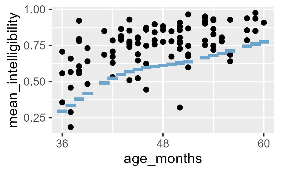
Intelligibility data with points from the 10th percentile line
If we ask GAMLSS to give us centiles for those gaps—herein lies the problem—we might get a warning message like the following:
centiles2 <- data_intel %>%
  select(age_months) %>%
  tidyr::expand(age_months = tidyr::full_seq(age_months, 1)) %>%
  wisclabmisc::predict_centiles(model)
#> Warning in predict.gamlss(obj, what = "mu", newdata = newx, type = "response", : There is a discrepancy  between the original and the re-fit
#>  used to achieve 'safe' predictions
#>
I don’t want to mess around in unsafe territory with GAMLSS. (What if they change how they handle this problem in the future?) So I would like to estimate values for those missing x values from the spline by hand.
Solution
Use predict() on the spline object to get the values
of the basis functions at the new x values. I stashed
the original spline object inside of the model.
mu_basis <- model$.user$mu_basis
ages_to_predict <- data_intel %>%
  tidyr::expand(age_months = tidyr::full_seq(age_months, 1))

mu_basis2 <- predict(mu_basis, newx = ages_to_predict$age_months)

library(patchwork)
tjmisc::ggmatplot(mu_basis) +
  tjmisc::ggmatplot(mu_basis2)
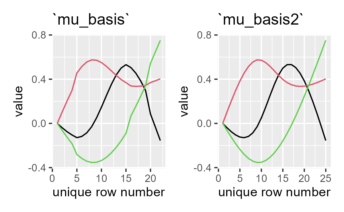
Basis functions for observed data (left) and the age range (right). The full age range is a little bit smoother than the observed data.
We do the following to get model parameters at each age. This code is the point of this note.
mu_basis <- model$.user$mu_basis
sigma_basis <- model$.user$sigma_basis
newx <- ages_to_predict$age_months

mu_basis2 <- cbind(1, predict(mu_basis, newx = newx))
sigma_basis2 <- cbind(1, predict(sigma_basis, newx = newx))

manual_centile <- tibble::tibble(
  age_months = newx,
  # multiply coefficients and undo link function
  mu = plogis(mu_basis2 %*% coef(model, what = "mu"))[, 1],
  sigma = plogis(sigma_basis2 %*% coef(model, what = "sigma"))[, 1],
  # now take centiles
  c10 = gamlss.dist::qBE(.1, mu, sigma)
)
manual_centile
#> # A tibble: 25 × 4
#>    age_months    mu sigma   c10
#>         <dbl> <dbl> <dbl> <dbl>
#>  1         36 0.522 0.341 0.294
#>  2         37 0.560 0.334 0.336
#>  3         38 0.596 0.328 0.378
#>  4         39 0.630 0.321 0.418
#>  5         40 0.661 0.315 0.456
#>  6         41 0.688 0.309 0.491
#>  7         42 0.712 0.304 0.522
#>  8         43 0.731 0.298 0.548
#>  9         44 0.745 0.293 0.569
#> 10         45 0.755 0.288 0.584
#> # ℹ 15 more rows
Let’s look at our manually computed 10th percentile versus the package-provided one.
ggplot(data_intel) +
  aes(x = age_months, y = mean_intelligibility) +
  geom_point() +
  geom_point(
    aes(y = c10),
    data = manual_centile,
    color = "orange",
    size = 10,
    shape = "+"
  ) +
  geom_point(
    aes(y = c10),
    data = centiles,
    color = "skyblue3",
    size = 10,
    shape = "-"
  ) +
  scale_x_continuous(breaks = c(36, 48, 60))
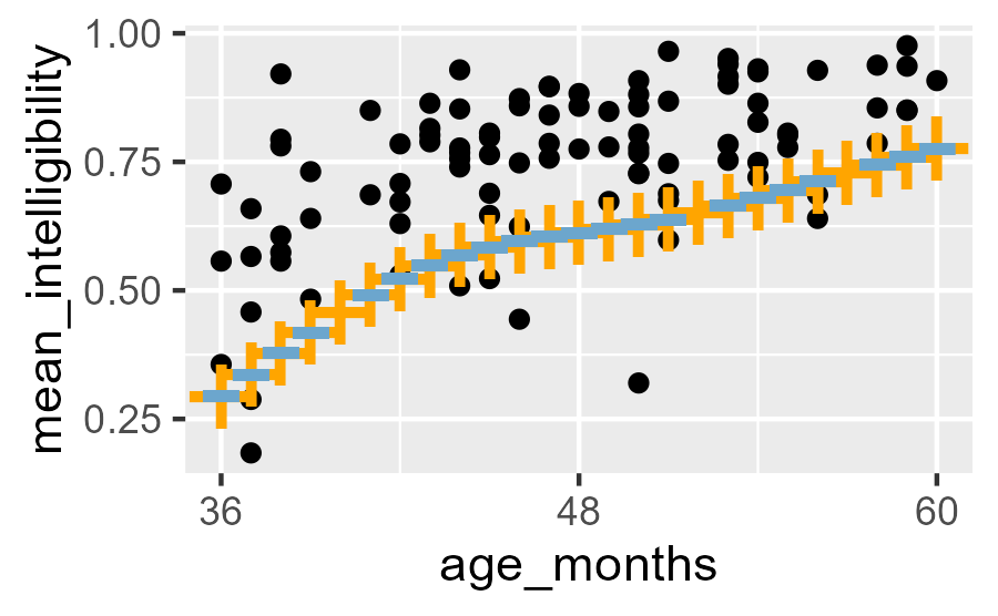
Intelligibility data with points from the 10th percentile line provided by `centiles.pred()` (blue hyphens) and computed by hand (orange pluses).
Leave a comment