A few days ago, I watched a terrific lecture by Bob Carpenter on Bayesian models. He started with a Bayesian approach to Fisher’s exact test. I had never heard of this classical procedure, so I was curious to play with the example. In this post, I use the same data that he used in the lecture and in an earlier, pre-Stan blog post. I show how I would go about fitting the model in Stan and inspecting the results in R.
Problem statement
We observed the following data.
| sex | n left handed | n right handed |
|---|---|---|
| male | 9 | 43 |
| female | 4 | 44 |
Question: Is the rate of left-handedness different between the male and female groups? Specifically, is left-handedness more likely in the male group?
Classical approach
In frequentist statistics, we might run Fisher’s exact test. At least, that’s what the flow charts tell us. To do that, we first put the data in a matrix.
# Create a matrix representation of the data for the fisher test
m <- matrix(
  c(9, 43, 4, 44),
  nrow = 2,
  byrow = TRUE,
  dimnames = list(
    sex = c("male", "female"),
    handedness = c("left", "right"))
  )
m
#>         handedness
#> sex      left right
#>   male      9    43
#>   female    4    44
We can run the two-tailed test: Are the two groups different?
fisher.test(m)
#>
#> 	Fisher's Exact Test for Count Data
#>
#> data:  m
#> p-value = 0.2392
#> alternative hypothesis: true odds ratio is not equal to 1
#> 95 percent confidence interval:
#>   0.582996 10.927993
#> sample estimates:
#> odds ratio
#>   2.283832
The output is a little verbose, but I do like how it spells out a sentence describing the alternative hypothesis.
We can also consider one-sided test: Is left-handedness greater in the male group?
fisher.test(m, alternative = "greater")
#>
#> 	Fisher's Exact Test for Count Data
#>
#> data:  m
#> p-value = 0.1502
#> alternative hypothesis: true odds ratio is greater than 1
#> 95 percent confidence interval:
#>  0.7006563       Inf
#> sample estimates:
#> odds ratio
#>   2.283832
In both tests, we cannot reject the null hypothesis because the p-value is greater than .05 ❌, so we would conclude that the two groups are not different.
But I don’t really know this test that well. We never covered it in any
of my stats classes, and indeed, this post is the first time I ever used
the function fisher.test(). If I had never heard of the test, I am not
quite sure what I would have done. Maybe a logistic regression (p =
.191 ❌).
Creating a Stan model
I’m very not fluent in the classical bag of tricks, but that’s okay. I know some Stan, I have an idea about how the data could have been generated, and that’s good enough ☺️. I can just write down my data-generating story in a model and let Stan compute a posterior distribution for the difference in handedness rates between the two groups.
For my model, I’m going to suppose that in each group, there is a probability of being left-handed called θ and that the counts we see result from a binomial process. The 9 left-handed males we observe are the number of successes from 52 observations of a process that “succeeds” with probability θmale.
To fit the model, we need a prior distribution. The prior’s job is to generate possible θ’s, and we will use our data to update the prior. The Beta distribution generates values between 0 and 1, so it’s an obvious choice.
In math, the model for a group would be:
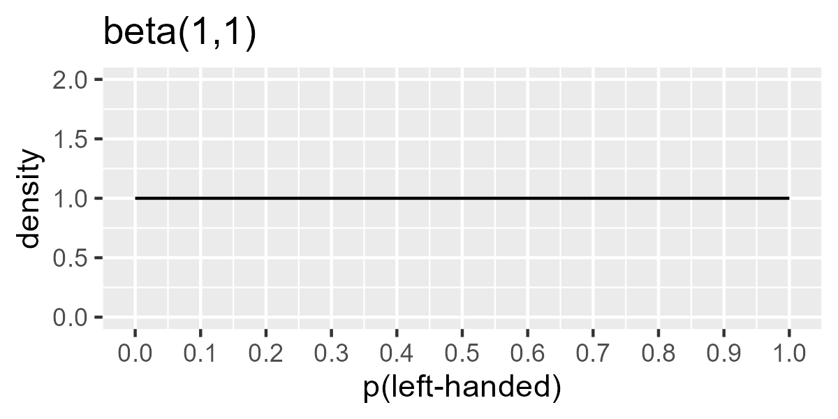
\[\begin{align*} n_\text{left-handed in group} &\sim \text{Binomial}(n_\text{total in group}, \theta_\text{group}) &\text{[likelihood]}\\ \theta_\text{group} &\sim \text{Beta}(a, b) &\text{[prior prob. of left-handedness]}\\ a, b &: \text{shape terms for prior} \end{align*}\]We can use a flat, uninformative prior by using a = 1, b = 1. This prior considers all probabilities from 0 to 1 as equally plausible.
library(ggplot2)
steps <- seq(from = 0, to = 1, by = .01)

ggplot(data.frame(x = steps, y = dbeta(steps, shape1 = 1, shape2 = 1))) +
  geom_line(aes(x, y)) +
  scale_x_continuous(breaks = (0:10) / 10) +
  ylim(0, 2) +
  labs(x = "p(left-handed)", y = "density", title = "beta(1,1)")
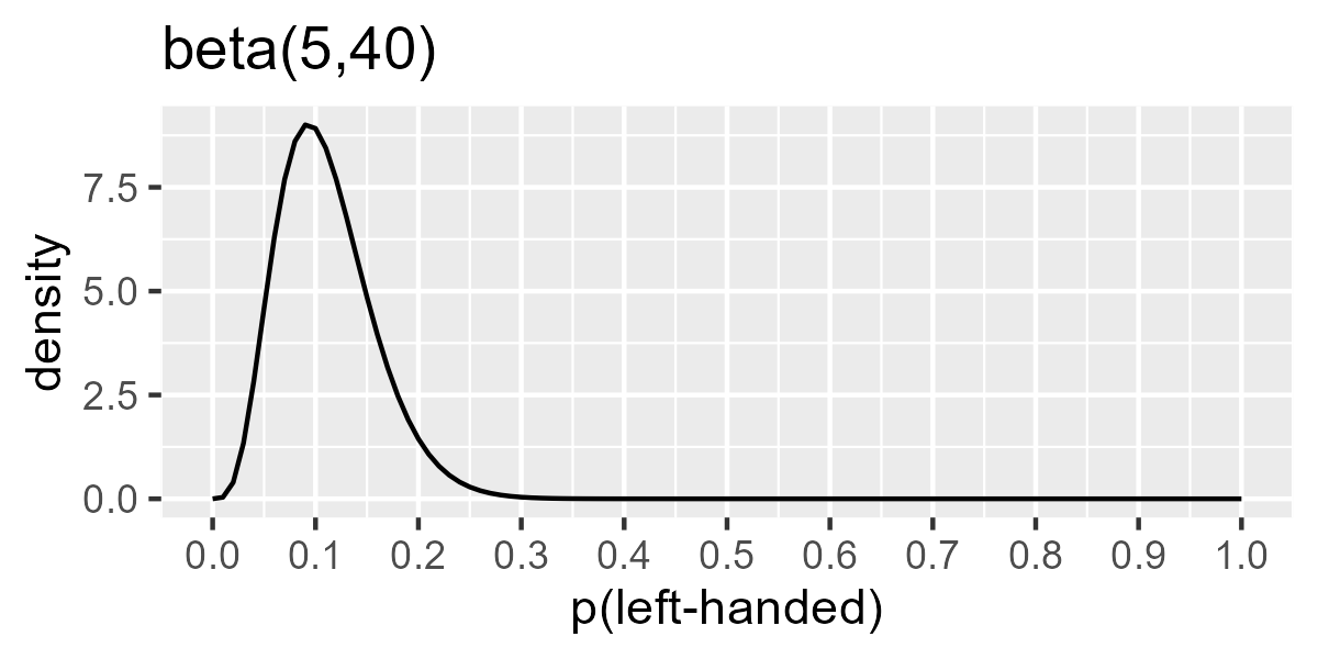
But I also think that 10-ish% of people are left handed. (I don’t know
where I first heard this number, but it’ll serve as my prior
information.) I toyed around with shape1 and shape2 parameters in
dbeta() until I got the prior Beta(5, 40), which is peaked around
.1-ish but wide enough to keep .5 and .15 as plausible values too.
ggplot(data.frame(x = steps, y = dbeta(steps, shape1 = 5, shape2 = 40))) +
  geom_line(aes(x, y)) +
  scale_x_continuous(breaks = (0:10) / 10) +
  labs(x = "p(left-handed)", y = "density", title = "beta(5,40)")
Let’s write out a really simple model in Stan. Okay, it used to be
really simple. Then I made the parameters for the Beta prior data
values, and then I created an option to just sample the prior
distribution. But the core of it is simple. The most important lines are
the one with ~ symbols. These correspond to the sampling statements in
the mathematical description of the model.
model_code <- "
data {
  int<lower=0> beta_a;
  int<lower=0> beta_b;
  int<lower=0> n_total_1;
  int<lower=0> n_total_2;
  int<lower=0> n_hits_1;
  int<lower=0> n_hits_2;
  int<lower=0, upper=1> sample_prior_only;
}
parameters {
  real<lower=0, upper=1> theta_1;
  real<lower=0, upper=1> theta_2;
}
model {
  theta_1 ~ beta(beta_a, beta_b);
  theta_2 ~ beta(beta_a, beta_b);

  if (sample_prior_only != 1) {
    n_hits_1 ~ binomial(n_total_1, theta_1);
    n_hits_2 ~ binomial(n_total_2, theta_2);
  }
}
generated quantities {
  real diff;
  diff = theta_1 - theta_2;
}
"
The generated quantities block runs on every sample of the posterior
distribution. Here, we compute the θmale −
θfemale on every draw. Computing the difference inside the
model code means that Stan will treat the diff values like any other
parameter of the model. It will show up in summary functions and in
plots of model parameters. That saves us some work later on.
Update: Migrated to cmdstanr. This post was originally written in 2017 and used the rstan interface to compile Stan models from R. I have updated this post to use the cmdstanr interface instead. I have kept around the original rstan code in place, albeit commented out. [May 26, 2022]
# # 2017 rstan-based version
# library(rstan)

# 2022 cmdstanr version
library(cmdstanr)
#> This is cmdstanr version 0.5.2
#> - CmdStanR documentation and vignettes: mc-stan.org/cmdstanr
#> - CmdStan path: C:/Users/Tristan/Documents/.cmdstan/cmdstan-2.29.2
#> - CmdStan version: 2.29.2
I begin by compiling the model. This step will create an executable program that can sample from the model. I do the compilation in its own step so that I can re-use the program for different versions of the model.
# # 2017 rstan-based version
# model_program <- stan_model(model_code = model_code)

# 2022 cmdstanr version
file <- write_stan_file(model_code, dir = "_caches", basename = "bfet")
model_program <- cmdstan_model(file)
For convenience, I wrote a function that fits different versions of this
model. This step is not necessary, but I don’t like repeating myself.
(Normally, you would use sampling(model_program, stan_data) with rstan or
model_program$sample(stan_data) with cmdstanr to get samples from a
model-program.)
run_model <- function(beta_a, beta_b, sample_prior_only) {
  stan_data <- list(
    beta_a = beta_a,
    beta_b = beta_b,
    n_total_1 = 9 + 43,
    n_total_2 = 4 + 44,
    n_hits_1 = 9,
    n_hits_2 = 4,
    sample_prior_only = sample_prior_only
  )

  # # 2017 rstan-based version
  #
  # # Use quietly() to hide the sampler's output text
  # # model <- purrr::quietly(sampling)(model_program, stan_data)
  # model <- purrr::quietly(sampling)(model_program, stan_data)
  #
  # # But print any warnings that would have appeared
  # invisible(lapply(model$warnings, warning, call. = FALSE))
  #
  # model$result

  # 2022 cmdstanr version
  model <- model_program$sample(data = stan_data, refresh = 0)
  model
}
The actual left-handed versus right-handed numbers are hard-coded, but I
can adjust the parameters for the Beta prior and toggle between sampling
from the prior and the posterior. Stan normally prints out verbose
progress information but I suppress that by using purrr::quietly(). I
still want warnings, so I print them if they arise.
Checking our prior information
Now, let’s draw samples from the priors of each model. This step lets us check that our program works as expected. We know how the values should be distributed—we made up the numbers!
m_informative_pd <- run_model(beta_a = 5, beta_b = 40, sample_prior_only = 1)
#> Running MCMC with 4 sequential chains...
#>
#> Chain 1 finished in 0.0 seconds.
#> Chain 2 finished in 0.0 seconds.
#> Chain 3 finished in 0.0 seconds.
#> Chain 4 finished in 0.0 seconds.
#>
#> All 4 chains finished successfully.
#> Mean chain execution time: 0.0 seconds.
#> Total execution time: 0.8 seconds.
m_informative_pd
#>  variable   mean median   sd  mad     q5    q95 rhat ess_bulk ess_tail
#>   lp__    -32.42 -32.09 1.03 0.72 -34.48 -31.45 1.00     1996     2506
#>   theta_1   0.11   0.11 0.05 0.05   0.05   0.20 1.00     3854     2857
#>   theta_2   0.11   0.11 0.05 0.04   0.05   0.20 1.00     3248     2659
#>   diff      0.00   0.00 0.07 0.06  -0.11   0.11 1.00     3607     2889

m_flat_pd <- run_model(beta_a = 1, beta_b = 1, sample_prior_only = 1)
#> Running MCMC with 4 sequential chains...
#>
#> Chain 1 finished in 0.0 seconds.
#> Chain 2 finished in 0.0 seconds.
#> Chain 3 finished in 0.0 seconds.
#> Chain 4 finished in 0.0 seconds.
#>
#> All 4 chains finished successfully.
#> Mean chain execution time: 0.0 seconds.
#> Total execution time: 0.6 seconds.
m_flat_pd
#>  variable  mean median   sd  mad    q5   q95 rhat ess_bulk ess_tail
#>   lp__    -4.01  -3.68 1.15 0.91 -6.26 -2.85 1.00     1709     1980
#>   theta_1  0.50   0.50 0.29 0.38  0.05  0.95 1.00     2919     2042
#>   theta_2  0.50   0.50 0.29 0.37  0.05  0.96 1.00     3053     2330
#>   diff     0.00   0.00 0.41 0.44 -0.68  0.68 1.00     3438     3009
We can confirm (by inspecting the diff row) that the difference in
left-handedness in both groups is 0 according to our priors. The
informative prior says that the values between 0.04 and
0.22 are plausible rates of left-handedness in each group.
It’s worth a moment to reflect on how obviously wrong the uninformative prior is. The central θ value in each group is .5. Therefore, half of the prior samples assert that there are more left-handed individuals than right-handed ones! If there is anything we know about handedness, it’s that left-handedness is less common than right-handedness. Uninformative sometimes connotes “unbiased” or “letting the data speak for itself”, but in this case, I would say “gullible”.
Sampling the posterior
Now, the fun part. We update our prior information with our data.
m_informative <- run_model(beta_a = 5, beta_b = 40, sample_prior_only = 0)
#> Running MCMC with 4 sequential chains...
#>
#> Chain 1 finished in 0.0 seconds.
#> Chain 2 finished in 0.0 seconds.
#> Chain 3 finished in 0.0 seconds.
#> Chain 4 finished in 0.0 seconds.
#>
#> All 4 chains finished successfully.
#> Mean chain execution time: 0.0 seconds.
#> Total execution time: 0.6 seconds.
m_informative
#>  variable   mean median   sd  mad     q5    q95 rhat ess_bulk ess_tail
#>   lp__    -70.62 -70.29 1.04 0.72 -72.62 -69.65 1.00     1883     2310
#>   theta_1   0.14   0.14 0.04 0.03   0.09   0.20 1.00     3057     2417
#>   theta_2   0.10   0.09 0.03 0.03   0.05   0.15 1.00     2798     2196
#>   diff      0.05   0.05 0.05 0.04  -0.03   0.12 1.00     3044     2559

m_flat <- run_model(beta_a = 1, beta_b = 1, sample_prior_only = 0)
#> Running MCMC with 4 sequential chains...
#>
#> Chain 1 finished in 0.0 seconds.
#> Chain 2 finished in 0.0 seconds.
#> Chain 3 finished in 0.0 seconds.
#> Chain 4 finished in 0.0 seconds.
#>
#> All 4 chains finished successfully.
#> Mean chain execution time: 0.0 seconds.
#> Total execution time: 0.6 seconds.
m_flat
#>  variable   mean median   sd  mad     q5    q95 rhat ess_bulk ess_tail
#>   lp__    -43.15 -42.82 1.02 0.73 -45.23 -42.18 1.00     1853     2211
#>   theta_1   0.18   0.18 0.05 0.05   0.11   0.28 1.00     3454     2414
#>   theta_2   0.10   0.09 0.04 0.04   0.04   0.18 1.00     3052     2393
#>   diff      0.08   0.08 0.07 0.07  -0.03   0.19 1.00     3525     2802
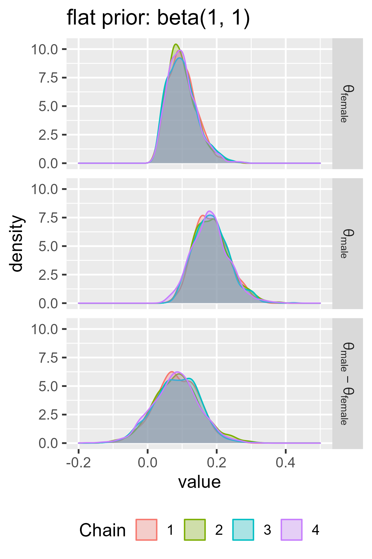
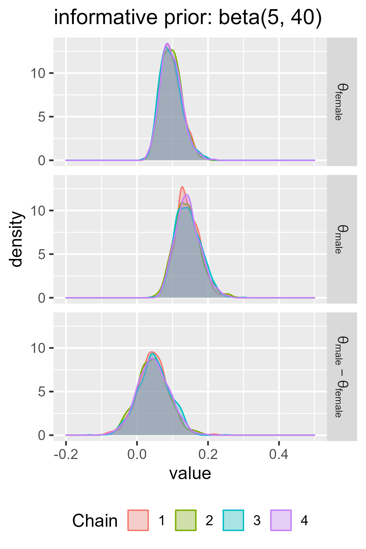
The flat model puts the difference at 0.08 and 90% of the plausible values fall in the interval [-0.03, 0.19]. The informative model is more skeptical of higher left-handedness rates, so it puts the difference at 0.05 with 90% of the values between [-0.03, 0.12]. Both of these intervals contain 0 and negative values ❌, so there is not much evidence for higher left-handedness in the male group.
To compute a “Bayesian p-value”, we could ask what proportion of differences are 0 or negative. There are more proper ways to make this inference in a Bayesian framework, but this approach is the easiest and it works for a model this simple. If 10% of the plausible values for the group differences are negative, then we assign a 10% probability to a negative group difference.
mean(df_flat$diff <= 0)
#> [1] 0.104

mean(df_informative$diff <= 0)
#> [1] 0.1415
It’s also worth comparing the two models. I’ve recently become a fan of
the ggmcmc package for quick
visualization of Stan models. The package uses a function ggs() to
create a long dataframe of MCMC samples. Then you plug those dataframes
into various plotting functions that start with ggs_. I especially
like how the package returns a plain ggplot2 plot that I can easily
adjust with a few extra lines of code.
For example, not much effort is required—after some practice and trial-and-error, of course—to visualize the posterior samples in each model.
library(ggmcmc)

# A helper dataframe for relabeling parameters. I'm writing them in a way that
# works with ?plotmath conventions.
labels <- data.frame(
  Parameter = c("theta_1", "theta_2", "diff"),
  Label = c("theta[male]", "theta[female]", "theta[male] - theta[female]")
)

# # 2017 rstan-based version
# a <- m_flat
# b <- m_informative

# 2022 cmdstanr version
a <- as_mcmc.list(m_flat)
b <- as_mcmc.list(m_informative)

# Get ggmcmc's tidy dataframe of each model.
# ggs() doesn't like that labels I made have brackets so I am suppressing its
# warnings.
ggs_flat <- suppressWarnings(
  ggs(a, description = "flat", par_labels = labels)
)
ggs_informative <- suppressWarnings(
  ggs(b, description = "informative", par_labels = labels)
)

# Remove log-posterior density if it sneaks in
ggs_flat <- ggs_flat[ggs_flat$Parameter != "lp__", ]
ggs_informative <- ggs_informative[ggs_informative$Parameter != "lp__", ]

ggs_density(ggs_flat) +
  facet_grid(Parameter ~ ., labeller = label_parsed) +
  ggtitle("flat prior: beta(1, 1)") +
  theme_grey(base_size = 14) +
  theme(legend.position = "bottom") +
  # so the two models can be compared
  xlim(-.2, .5)

ggs_density(ggs_informative) +
  facet_grid(Parameter ~ ., labeller = label_parsed) +
  ggtitle("informative prior: beta(5, 40)") +
  theme_grey(base_size = 14) +
  theme(legend.position = "bottom") +
  # so the two models can be compared
  xlim(-.2, .5)
We can also compare the models together in a single plot by passing a
list of model dataframes into ggs_caterpillar().
ggs_caterpillar(
  D = list(ggs_flat, ggs_informative),
  line = 0,
  thick_ci = c(0.05, 0.95),
  thin_ci = c(0.025, 0.975)
) +
  # Parse the labels as formatted math
  scale_y_discrete(
    breaks = as.character(unique(ggs_flat$Parameter)),
    labels = parse(text = as.character(unique(ggs_flat$Parameter)))
  ) +
  labs(
    caption = "Intervals: thick 90%, thin 95%. Point: median.",
    y = NULL,
    x = NULL
  ) +
  theme_grey(base_size = 14)
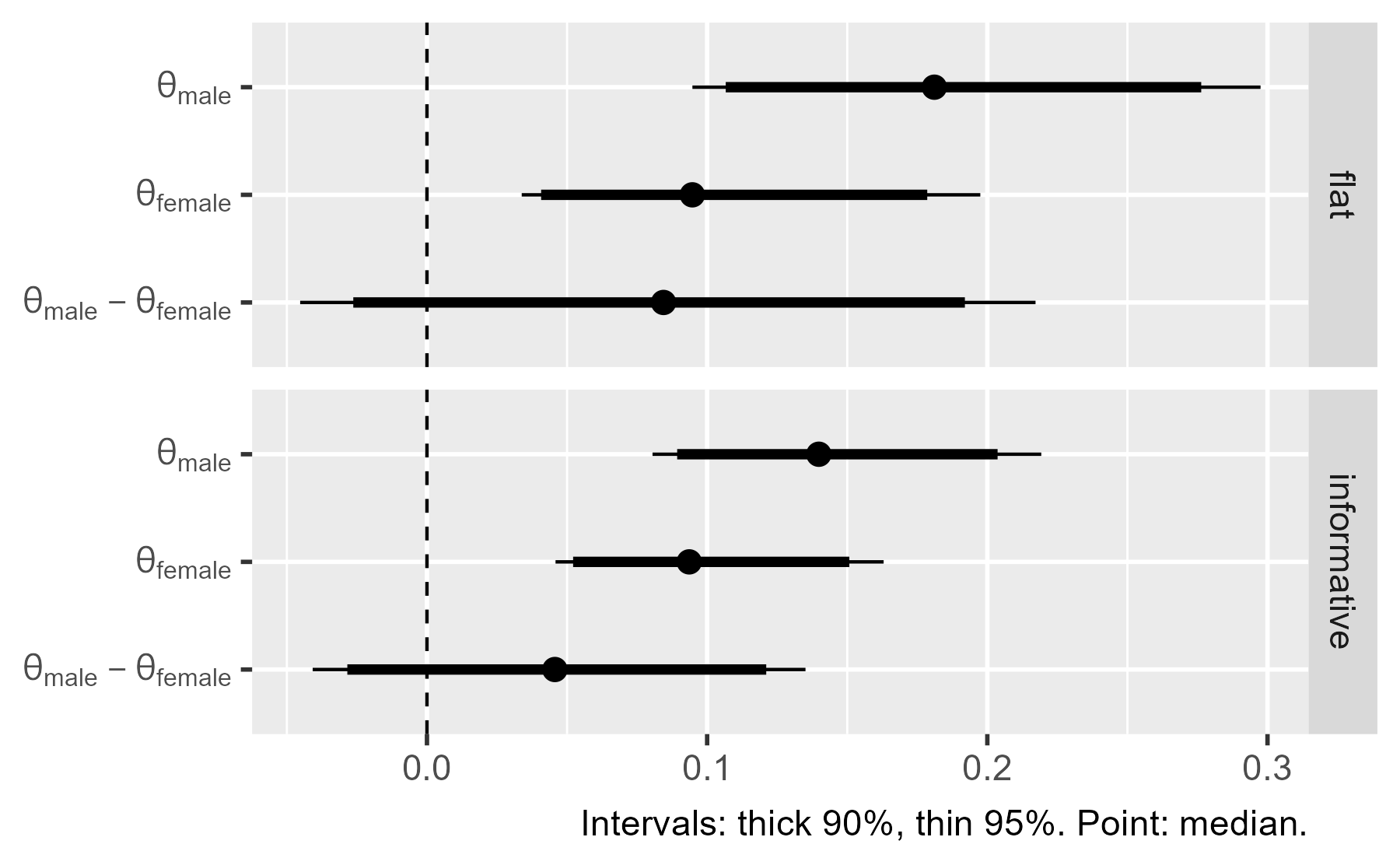
There’s a lot of useful information here. First, the intervals in the flat prior model are wider than the ones for the informative model. The two models largely agree on the values in the female group, although the flat prior model is wider. These wider intervals indicate greater uncertainty about the parameter values. The two models disagree on the male group, because the informative model assigns little prior probability to values greater than .25 but the flat model doesn’t discount those possibilities.
The models also demonstrate the regularizing effect of prior information. Regularization broadly refers to techniques to avoid overfitting a dataset. Priors can regularize a model by making it skeptical of certain parameter values—in this case, high values of left-handedness. The male probabilities in the flat model are basically pulled towards the values in the informative prior (.1-ish). We can see this effect in how the midpoint is shifted in the flat model versus the informative model.
I would be remiss if I didn’t end with the following disclaimer/trivia. In a way, the question behind this post is ill-posed because handedness is not quite a binary measure. Some years ago, I had a class on stuttering and fluency disorders. (I used to be a speech pathologist.) There once was a lot of research on the association between handedness and stuttering, and at some point, researchers figured out that they could measure handedness as a continuous measure. They gave people a survey asking which hands they use for certain tasks and then computed a so-called dextrality quotient from the responses. I had the concept driven home when I once saw my wife casually switch between her left and right hands while brushing her teeth. I would probably poke a hole through my cheek if I used my left hand! So: Handedness may be a matter of degree. (Or maybe not. I mostly wanted to mention the dextrality quotient. It’s fun to think about.)
Last knitted on 2022-05-27. Source code on GitHub.1
-
.session_info
#> ─ Session info ───────────────────────────────────────────────────────────────
#>  setting         value
#>  version         R version 4.2.0 (2022-04-22 ucrt)
#>  os              Windows 10 x64 (build 22000)
#>  system          x86_64, mingw32
#>  ui              RTerm
#>  language        (EN)
#>  collate         English_United States.utf8
#>  ctype           English_United States.utf8
#>  tz              America/Chicago
#>  date            2022-05-27
#>  pandoc          NA
#>  stan (cmdstanr) 2.29.2
#>
#> ─ Packages ───────────────────────────────────────────────────────────────────
#>  package        * version date (UTC) lib source
#>  abind            1.4-5   2016-07-21 [1] CRAN (R 4.2.0)
#>  assertthat       0.2.1   2019-03-21 [1] CRAN (R 4.2.0)
#>  backports        1.4.1   2021-12-13 [1] CRAN (R 4.2.0)
#>  checkmate        2.1.0   2022-04-21 [1] CRAN (R 4.2.0)
#>  cli              3.3.0   2022-04-25 [1] CRAN (R 4.2.0)
#>  cmdstanr       * 0.5.2   2022-05-01 [1] Github (stan-dev/cmdstanr@e9c12be)
#>  colorspace       2.0-3   2022-02-21 [1] CRAN (R 4.2.0)
#>  crayon           1.5.1   2022-03-26 [1] CRAN (R 4.2.0)
#>  data.table       1.14.2  2021-09-27 [1] CRAN (R 4.2.0)
#>  DBI              1.1.2   2021-12-20 [1] CRAN (R 4.2.0)
#>  digest           0.6.29  2021-12-01 [1] CRAN (R 4.2.0)
#>  distributional   0.3.0   2022-01-05 [1] CRAN (R 4.2.0)
#>  dplyr          * 1.0.9   2022-04-28 [1] CRAN (R 4.2.0)
#>  ellipsis         0.3.2   2021-04-29 [1] CRAN (R 4.2.0)
#>  evaluate         0.15    2022-02-18 [1] CRAN (R 4.2.0)
#>  fansi            1.0.3   2022-03-24 [1] CRAN (R 4.2.0)
#>  farver           2.1.0   2021-02-28 [1] CRAN (R 4.2.0)
#>  generics         0.1.2   2022-01-31 [1] CRAN (R 4.2.0)
#>  GGally           2.1.2   2021-06-21 [1] CRAN (R 4.2.0)
#>  ggmcmc         * 1.5.1.1 2021-02-10 [1] CRAN (R 4.2.0)
#>  ggplot2        * 3.3.6   2022-05-03 [1] CRAN (R 4.2.0)
#>  git2r            0.30.1  2022-03-16 [1] CRAN (R 4.2.0)
#>  glue             1.6.2   2022-02-24 [1] CRAN (R 4.2.0)
#>  gtable           0.3.0   2019-03-25 [1] CRAN (R 4.2.0)
#>  here             1.0.1   2020-12-13 [1] CRAN (R 4.2.0)
#>  highr            0.9     2021-04-16 [1] CRAN (R 4.2.0)
#>  jsonlite         1.8.0   2022-02-22 [1] CRAN (R 4.2.0)
#>  knitr          * 1.39    2022-04-26 [1] CRAN (R 4.2.0)
#>  labeling         0.4.2   2020-10-20 [1] CRAN (R 4.2.0)
#>  lifecycle        1.0.1   2021-09-24 [1] CRAN (R 4.2.0)
#>  magrittr         2.0.3   2022-03-30 [1] CRAN (R 4.2.0)
#>  matrixStats      0.62.0  2022-04-19 [1] CRAN (R 4.2.0)
#>  munsell          0.5.0   2018-06-12 [1] CRAN (R 4.2.0)
#>  pillar           1.7.0   2022-02-01 [1] CRAN (R 4.2.0)
#>  pkgconfig        2.0.3   2019-09-22 [1] CRAN (R 4.2.0)
#>  plyr             1.8.7   2022-03-24 [1] CRAN (R 4.2.0)
#>  posterior        1.2.1   2022-03-07 [1] CRAN (R 4.2.0)
#>  processx         3.5.3   2022-03-25 [1] CRAN (R 4.2.0)
#>  ps               1.7.0   2022-04-23 [1] CRAN (R 4.2.0)
#>  purrr            0.3.4   2020-04-17 [1] CRAN (R 4.2.0)
#>  R6               2.5.1   2021-08-19 [1] CRAN (R 4.2.0)
#>  ragg             1.2.2   2022-02-21 [1] CRAN (R 4.2.0)
#>  RColorBrewer     1.1-3   2022-04-03 [1] CRAN (R 4.2.0)
#>  Rcpp             1.0.8.3 2022-03-17 [1] CRAN (R 4.2.0)
#>  reshape          0.8.9   2022-04-12 [1] CRAN (R 4.2.0)
#>  rlang            1.0.2   2022-03-04 [1] CRAN (R 4.2.0)
#>  rprojroot        2.0.3   2022-04-02 [1] CRAN (R 4.2.0)
#>  rstudioapi       0.13    2020-11-12 [1] CRAN (R 4.2.0)
#>  scales           1.2.0   2022-04-13 [1] CRAN (R 4.2.0)
#>  sessioninfo      1.2.2   2021-12-06 [1] CRAN (R 4.2.0)
#>  stringi          1.7.6   2021-11-29 [1] CRAN (R 4.2.0)
#>  stringr          1.4.0   2019-02-10 [1] CRAN (R 4.2.0)
#>  systemfonts      1.0.4   2022-02-11 [1] CRAN (R 4.2.0)
#>  tensorA          0.36.2  2020-11-19 [1] CRAN (R 4.2.0)
#>  textshaping      0.3.6   2021-10-13 [1] CRAN (R 4.2.0)
#>  tibble         * 3.1.7   2022-05-03 [1] CRAN (R 4.2.0)
#>  tidyr          * 1.2.0   2022-02-01 [1] CRAN (R 4.2.0)
#>  tidyselect       1.1.2   2022-02-21 [1] CRAN (R 4.2.0)
#>  utf8             1.2.2   2021-07-24 [1] CRAN (R 4.2.0)
#>  vctrs            0.4.1   2022-04-13 [1] CRAN (R 4.2.0)
#>  withr            2.5.0   2022-03-03 [1] CRAN (R 4.2.0)
#>  xfun             0.31    2022-05-10 [1] CRAN (R 4.2.0)
#>
#>  [1] C:/Users/Tristan/AppData/Local/R/win-library/4.2
#>  [2] C:/Program Files/R/R-4.2.0/library
#>
#> ──────────────────────────────────────────────────────────────────────────────

Leave a comment