Chapter 11 Development of referent selection
11.1 Nonwords versus familiar words
I asked whether the recognition of familiar words differed from the fast selection of referents for nonwords. I fit a Bayesian, mixed effects logistic regression, growth curve model, as in Chapter 5. For the real word and nonword conditions, there is a well-defined target image: the familiar image for real words and the novel/unfamiliar image for nonwords. The outcome measures were the probabilities of fixating to the target image in each condition:
- P(look to familiar image | hear a real word)
- P(look to unfamiliar image | hear a nonword)
Both the real word and nonword conditions measure referent selection as the probability of fixating on the appropriate referent when presented with a label. The important analytic question is whether and to what degree these two probabilities differ. The growth curve model is similar to the one in Chapter 5 with linear, quadratic and cubic time features but it adds a condition effect which interacts with these features. The linear model was:
\[ \small \begin{align*} \text{log\,odds}(\text{looking}) =\ &\beta_0 + \beta_1\text{Time}^1 + \beta_2\text{Time}^2 + \beta_3\text{Time}^3\ + &\text{[nonword curve]} \\ (&\gamma_0 + \gamma_1\text{Time}^1 + \gamma_2\text{Time}^2 + \gamma_3\text{Time}^3)*\text{Condition} \ &\text{[real words]} \\ \end{align*} \normalsize \]
I fit a separate model for each year of the study. Appendix D contains the R code used to fit these models along with a description of the specifications represented by the model syntax. The mixed model included by-child and by-child-by-condition random effects to allow some of a child’s growth curve features to be similar between conditions (by-child effects) and to differ between conditions (by-child-by-condition effects).
For these analyses, I limited focus to distractor-initial trials, and modeled the data from 300 to 1500 ms after target onset. I removed any Age × Child levels if a child had fewer than 4 fixations in a single time bin. In other words, children had to have at least 4 looks to one of the images in every 50 ms time bin. This screening removed 13 children at age 3, 15 at age 4, and 6 at age 5.
Figure 11.1 shows the group averages of the growth curves. For each condition and age, I computed the empirical growth curve for each participant, and I averaged the participants’ growth curves together to obtain group averages. I also applied this process to 100 model-estimated growth curves.
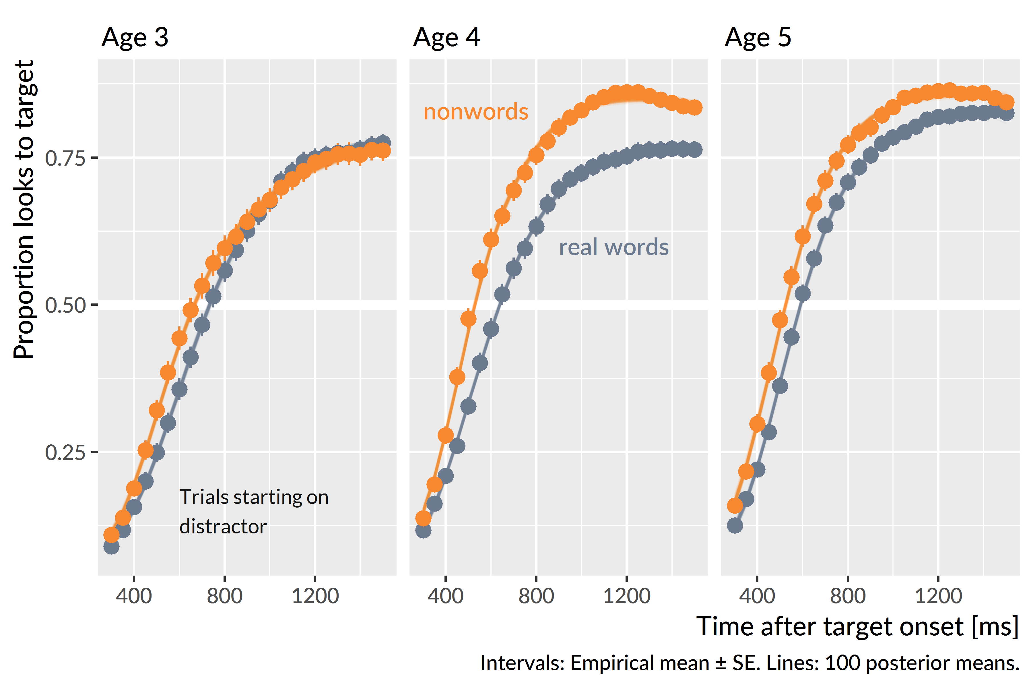
Figure 11.1: Averages of participants’ growth curves in each condition and age. The lines represent 100 posterior predictions of the group average.
In Chapter 5, I claim that for these growth curve models only the intercept and linear time terms are behaviorally meaningful model parameters. The intercept measures the average growth curve value so it reflects overall looking reliability, and the linear time term measures the overall steepness of the growth so it reflects lexical processing efficiency. I also derived a measure of peak looking probability by taking the median of top five points in a growth curve, and this peak provides a measure of word recognition certainty. Higher peaks indicate less uncertainty about a word.
I evaluated the general condition effects by looking at how the population-level (“fixed”) effects differed in each condition. Due to ceiling effects, where children’s growth curves saturated 100% looking probabilities, the population-level average growth curve outperformed the observed group averages in Figure 11.1. The condition differences described by these population-level effects, however, do qualitatively match the patterns in the group averages.
The two conditions did not reliably differ at age 3. The population-level average proportion of looks to the target for nonwords was .60 [90% UI: .55, .65], compared to .56 [.51, .60] for real words—a difference (nonword advantage) of .05 [−.01, .11]. For the linear time feature, the nonword slope increases by 9.00% [−1.00%, 18.0%] in the real word condition. Both these 90% intervals include 0 as a plausible estimate for the condition difference, so there is uncertainty about the sign of the effect. I therefore conclude that the conditions did not credibly differ on average at age 3.
There was an advantage for the nonword condition at age 4 and age 5. The population-level average proportion of looks for the nonwords was .79 [90% UI: .76, .82], compared to .62 [.58, .66] for real words. On average, children looked less to target for the real words than the nonwords. There was a suggestive linear time effect where the nonword curve was 13.0% [1.00%, 25.0%] steeper than the real word one. The curve for real words was probably less steep at age 4 but small values near 0 remain plausible. At age 5, only the average probability difference was credible, .81 [90% UI: .78, .83] for nonwords compared to .72 [.68, .75] for real words. In general, children performed better in the nonword condition than the real word condition at age 4 and age 5. This difference shows up in the growth curve model through intercept effects, although it is plausible that children’s nonword growth curves were steeper than the real word curves at age 4.
I analyzed the children’s model-estimated growth curve peaks. Each posterior sample of the model represents a plausible set of growth curve parameters for the data, so for each of these samples, I calculated the growth curves for each child and the peaks of the growth curves. Figure 11.2 shows the posterior averages of the growth curves peaks for each participant.
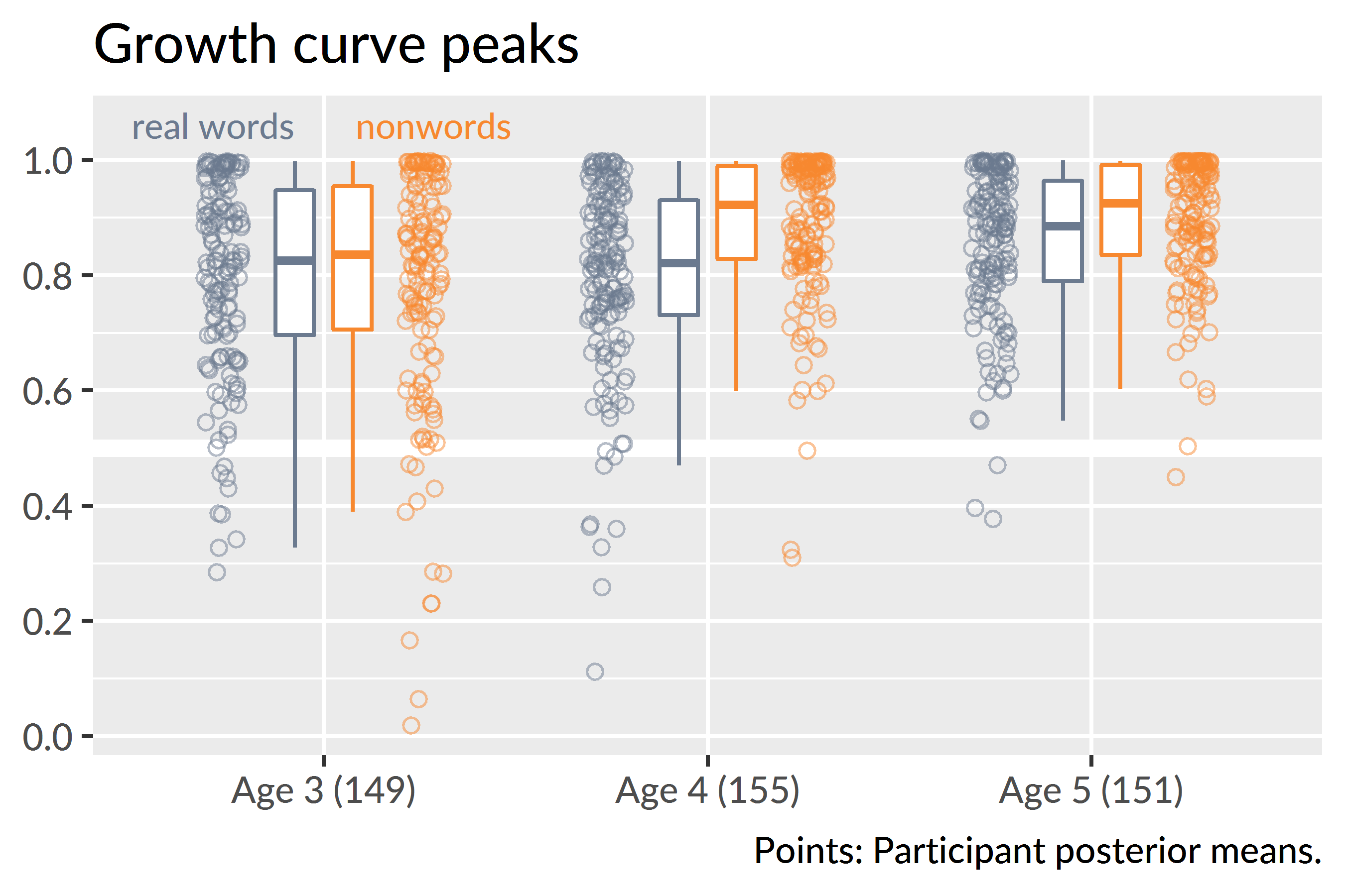
Figure 11.2: Growth curve peaks by child, condition and year of the study. The movement of the medians conveys how the nonword peaks effect increased from age 3 to age 4 and the real word peaks increased from age 4 to age 5. The piling of points near the 1.0 line depicts how children reached ceiling performance on this task.
Descriptive statistics reveal the developmental trends for this task. At age 3, the median peak values were similar for the two conditions: .84 for nonwords and .83 for real words. The peaks increased for the nonword condition in the following year with a median value of .92. It is worth emphasizing what this statistic tells us: At age 4, half of the children had a peak looking probability of .92 or greater. In other words, half the children performed near the ceiling on this task by age 4. At age 5, the median nonword peak was .93, essentially unchanged from age 4. For the real words, the median peak increased from .82 at age 4 to .89 at age 5.
To quantify the degree of ceiling performance, I calculated the number of children per condition with a growth curve peak greater than or equal to .99 over the posterior distribution. For the nonword condition, there were 23 [90% UI: 20, 26] children who performed at ceiling at age 3, 41 [36, 45] at age 4, 40 [36, 44] and at age 5. For the real word condition, the number of children attaining ceiling performance was more uneven: there were 20 [16, 24] ceiling-performers at age 3, 13 [10, 16] at age 4, and 26 [23, 29] at age 5.
To compare peaks looking probabilities between ages, I fit a linear mixed effects model with restricted maximum likelihood via the lme4 R package (vers. 1.1.18.1; Bates, Mächler, Bolker, & Walker, 2015). I regressed the children’s average growth curve peaks onto experimental condition, age group, and the age × condition interaction. The model included randomly varying intercepts for child and child × age. This modeling software does not provide p-values for its effects estimates, so for these comparisons, I decided that an effect was significant when the t statistic for a population-level (“fixed”) effect had an absolute value of 2 or greater. In practical terms, this convention interprets an effect as “significant” when its estimate is at least 2 standard errors away from 0. (Gelman & Hill, 2007 use this approach with mixed models.)
At age 3, the two conditions did not significantly differ, Breal−nonword = .01, t = 0.95. At age 4, nonword peaks were on average .09 proportion units greater than the real word peaks, t = 5.79, and at age 5, the nonword peaks were .04 proportion units greater than the real word peaks, t = 2.56. For the nonword condition there was a significant increase in the peaks from age 3 to age 4, B4−3 = .10, t = 5.99, whereas there was no improvement from age 4 to age 5, t = 0.37. In the real word condition, there was only a significant improvement from age 4 to age 5, B5−4 = .06, t = 3.25.
Finally, I asked whether expressive vocabulary size correlated with peak looking performance on the two conditions. Correlations among real word peaks, nonword peaks, expressive vocabulary and receptive vocabulary are given in Table 11.1. At all three years, children with larger vocabularies had higher nonword peak looking values. At age 3 and age 4, vocabulary positively correlated with real-word looking performance. Figure 11.3 illustrates the relationship between the peaks and expressive vocabulary. When there is more variability in the peaks, as at age 3, the vocabulary effect on the nonwords is strongest.
| Study | Real word peak | Nonword peak | PPVT-4 standard | |
|---|---|---|---|---|
| Age 3 | Nonword peak | r(149) = .24** | ||
| PPVT-4 standard | r(139) = .23** | r(139) = .46*** | ||
| EVT-2 standard | r(137) = .15 | r(137) = .30*** | r(137) = .69*** | |
| Age 4 | Nonword peak | r(155) = .29*** | ||
| PPVT-4 standard | r(152) = .15 | r(152) = .23** | ||
| EVT-2 standard | r(153) = .23** | r(153) = .20* | r(152) = .78*** | |
| Age 5 | Nonword peak | r(151) = .13 | ||
| EVT-2 standard | r(149) = −.06 | r(149) = .23** |
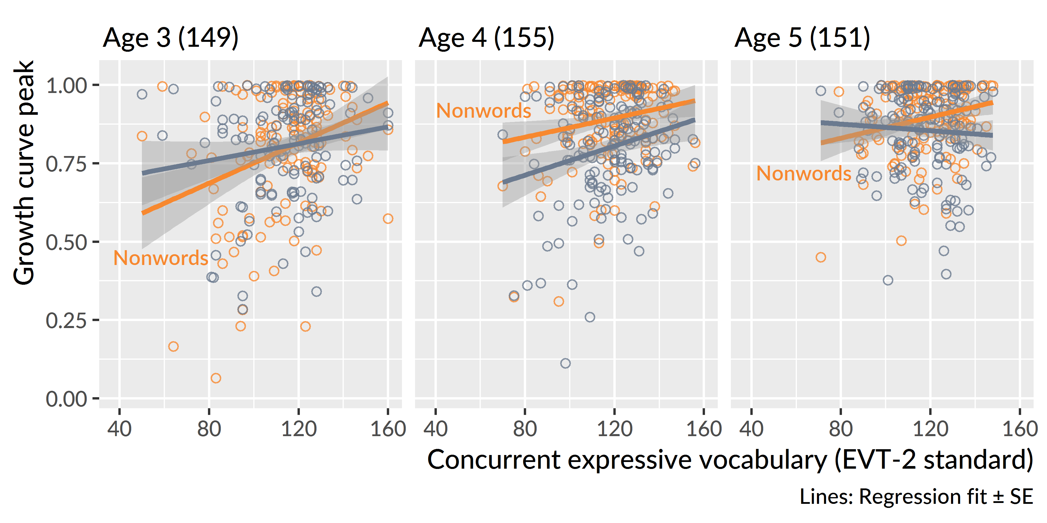
Figure 11.3: Relationships between expressive vocabulary and growth curve peaks at each age.
Summary. Children performed similarly for real words and nonwords at age 3. Children’s processing of nonwords improved at age 4. At this age, performance also began to saturate with the group average for peak looking probability greater than .9 for the nonword condition. Consequently, children did not improve in processing of nonwords from age 4 to age 5. For the real word condition, children’s performance did not change from age 3 to age 4 but it did improve from age 4 to age 5. At both age 4 and age 5, there was a decisive advantage for the nonword condition. Finally, children with larger expressive vocabularies looked more to the nonwords compared to children with smaller vocabularies. A comparable effect for real words was observed at age 3 and age 4 but only reliably observed at age 4.
11.2 Does age-3 referent selection better predict age-5 vocabulary?
I hypothesized that performance on the nonword condition would be a better predictor of future vocabulary size than the real word condition. This hypothesis follows from the assumption that fast referent selection, as opposed to familiar word recognition, is a more relevant skill for word-learning. Put another way, a child’s ability to quickly map a novel word to a referent is more closely related to the demands of in the moment word-learning than familiar word recognition.
In Chapter 5, I found that peak looking probability at age 3 positively correlated with age 5 vocabulary. Pairing this finding with my hypothesis, I predicted that the growth curve peaks in the nonword condition at age 3 would be better predictors of vocabulary at age 5 than the real word peaks at age 3.
For these analyses, I regressed age-5 expressive vocabulary (EVT-2) standard scores onto age-3 expressive vocabulary score and onto age-3 real word peaks or age-3 nonword peaks. There were 116 children with data available for this analysis. There was an expectedly strong relationship between age 3 and age 5 vocabulary, R2 = .49. A 1-SD (18-point) increase in vocabulary at age 3 predicted an 0.7-SD (10-point) increase at age 5. There was no effect of age-3 real-word peak over and above age-3 vocabulary, p = .59. There was a significant effect of the nonword peak, p = .005, ΔR2 = .03, over and above age-3 vocabulary. A .1 increase in nonword peak probability predicted a 0.10-SD (1.4-point) increase in age-5 vocabulary. Figure 11.4 depicts the difference between the two conditions with a flat line for the real condition and small slope for the nonword condition.
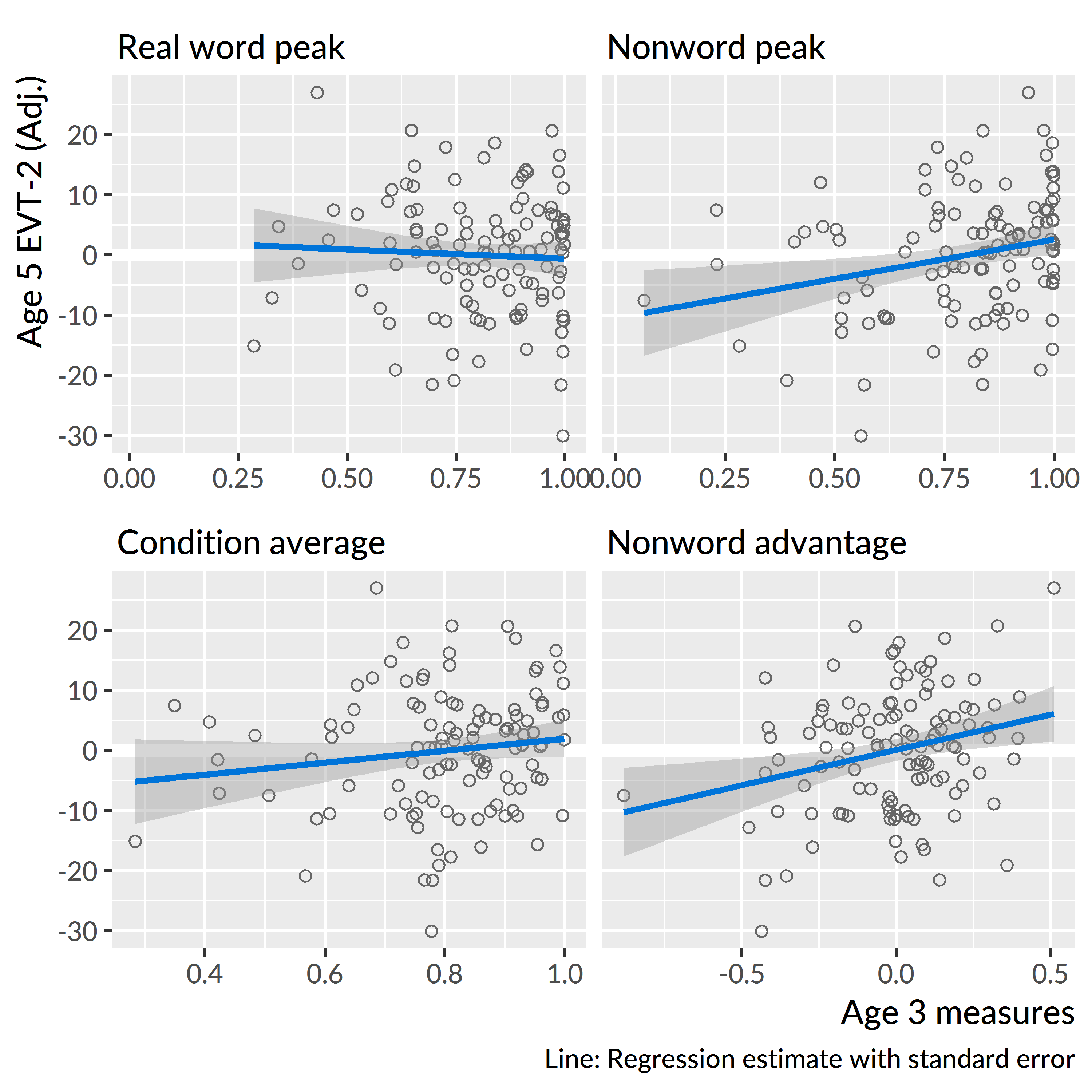
Figure 11.4: Marginal effects of age-3 referent selection measures on age-5 expressive vocabulary standard scores. The vocabulary scores were adjusted (residualized) to control for age-3 vocabulary, so these regression lines show the effects of the predictors over and above age-3 vocabulary.
Finally, I tested whether the difference between nonword and real word peaks within children predicted vocabulary growth. By themselves, differences do not convey much information about how well the child performed: A difference of 0 can happen if a child has peaks of .1 in both conditions or .9 in both conditions. To control for general referent selection performance, therefore, I also included the within-child averages of the two peaks. The model predicted age-5 vocabulary using the within-child average of the peaks, the nonword advantage, and age-3 vocabulary. In this case, condition-averaged performance did not significantly predict age-5 vocabulary, p = .22. The condition differences did predict age-5 vocabulary: A .1 increase in the nonword condition advantage predicted a 0.08-SD (1.1-point) increase in age-5 vocabulary, p = .009
Summary. A child’s performance in the nonword condition at age 3 positively predicted expressive vocabulary size at age 5. This effect held even when controlling age-3 vocabulary size, and the effect emerged when using the absolute growth curve peak or using the relative advantage of the nonword condition over the real word condition. Although the effects were significant, the effect sizes were small. The EVT-2 is normed to have an IQ-like scale with a mean of 100 and standard deviation of 15. An increase of .1 in age-3 growth curve peak predicted an increase in age-5 vocabulary of 1.4, approximately one tenth of the test norms’ standard deviation.
11.3 Discussion
Children showed developmental improvements in referent selection for the real word and nonword trials. The changes were not consistent year-over-year improvements however. Nonword processing improved from age 3 to age 4 and real word recognition improved from age 4 and to age 5. One reason for these limited improvements is that the two-image word recognition task was too easy. At age 4, approximately 25% of children had nonword growth curve peaks of .99 or greater.
Despite the presence of ceiling effects, vocabulary size had a small-to-medium positive correlation with nonword growth curve peaks at all three ages. Children who knew more words had a higher probability of looking to the novel object when presented with a nonword. This replicates the vocabulary advantage in processing nonwords observed by Bion et al. (2013) and Law and Edwards (2015). This effect is probably bidirectional with larger vocabularies making fast referent selection easier, and fast referent selection being a crucial mechanism for word-learning. To further examine the direction of effect, I tested whether nonword performance at age 3 predicted expressive vocabulary size at age 5. There was a small predictive effect where children with high nonword peaks had a larger vocabulary size two years later. Although real word and nonword performance had a small-to-medium positive correlation, children’s processing of the real words had no predictive value. Real word peaks did not predict vocabulary, nor did the average of real word and nonword peaks have an effect over and above the difference of the peaks. This result was unexpected, given how lexical processing can predict future language outcomes as in Chapter 5. On the other hand, familiar word recognition with a familiar object and novel object is probably not demanding enough for individual differences to predict future vocabulary size
For these two conditions, I hypothesized that word recognition in the real word condition would be easier than in the nonword condition, or failing that, the two conditions would not reliably differ. I had discounted a third possibility of any overall advantage for nonwords over real words. The advantage of nonwords at age 4 and age 5 over real words was therefore an unexpected result.
Why might children perform better on the nonword trials than the real words? The results are consistent with a novelty bias in referent selection (Horst et al., 2011; Mather & Plunkett, 2012). An additional factor may be the presence of the mispronunciation trials—reported in Chapter 12. The mispronunciations may undermine familiar word recognition. For one-third of the trials, children hear an imperfect version of a familiar word, and they show more uncertain responses to them. This environment may cause children to downweight the syllable-initial sounds. Such an adaptation would lead to lower overall activation of the real words. This possibility is a limitation of this study: A design with just real words and nonwords would provide a better comparison of the two kinds of words. Alternatively, the novelty bias could interfere with processing of familiar words. For some trials, children could have ignored the familiar word and focused attention on the novel object due to a novelty bias.
References
Bates, D., Mächler, M., Bolker, B., & Walker, S. (2015). Fitting linear mixed-effects models using lme4. Journal of Statistical Software, 67(1), 1–48. doi:10.18637/jss.v067.i01
Gelman, A., & Hill, J. (2007). Data analysis using regression and multilevel/hierarchical models. New York: Cambridge University Press.
Bion, R. A. H., Borovsky, A., & Fernald, A. (2013). Fast mapping, slow learning: Disambiguation of novel word–object mappings in relation to vocabulary learning at 18, 24, and 30 months. Cognition, 126(1), 39–53. doi:10.1016/j.cognition.2012.08.008
Law, F., II, & Edwards, J. R. (2015). Effects of vocabulary size on online lexical processing by preschoolers. Language Learning and Development, 11(4), 331–355. doi:10.1080/15475441.2014.961066
Horst, J. S., Samuelson, L. K., Kucker, S. C., & McMurray, B. (2011). What’s new? Children prefer novelty in referent selection. Cognition, 118(2), 234–244. doi:10.1016/j.cognition.2010.10.015
Mather, E., & Plunkett, K. (2012). The role of novelty in early word learning. Cognitive Science, 36(7), 1157–1177. doi:10.1111/j.1551-6709.2012.01239.x