Compute sensitivity and specificity scores from (weighted) observed data — compute_sens_spec_from

pROC::roc() does not support observation-weights when computing ROC curves. This function fills that gap.

Usage

compute_sens_spec_from_ecdf(
  data,
  response,
  predictor,
  weights = NULL,
  direction = NULL,
  levels = NULL
)

Arguments

data: a dataframe containing responses (groupings) and predictor variable
response: a bare column name with the group status (control vs. cases). If the response has more than two groups, the first element of levels is the control group and the second element of levels is the case group.
predictor: a bare column name with the predictor to use for classification
weights: a bare column name for the observation weights. If weights is set to NULL or not provided, all values receive equal weight and conventional sensitivity and specificity scores are returned.
direction: direction for computing case status. pROC::roc()'s direction conventions are supported: "<" (i.e., control < case) and ">" (control > case), or "auto" to have pROC guess the direction (if applicable). Alternatively, more verbose directions are supported: "case-low" or "control-high" if a low score predicts case status (case <= threshold < control, analogous to pROC's ">") and "case-high" or "control-low" if a high score predicts case status (control < threshold <= case, analogous to pROC's "<"). These directions are translated into the pROC conventions.
levels: two-element vector c(control, case) where control is the value of response for the control group and case is the value of response for the case group. The ordering matters: The first element of the vector names the control group.

Value

A dataframe of stepwise empirical ROC coordinates computed from (optionally weighted) data. The output includes columns for the predictor variable, .sensitivities, .specificities, .auc, .comparison, .n_controls, .n_cases, .w_controls, .w_cases, .comparison, .direction, .response, .controls, and .cases. n_ columns contain the number of observations for that predictor value and w_ contain the total weight of the observations for that predictor value.

Details

The .sensitivities and .specificities columns are calculated directly from the (weighted) ECDFs of the controls and cases, so no call to pROC::roc() is made.

.auc is calculated using trapezoid_auc().

c(-Inf, Inf) are added to the predictor vector so that sensitivities and specificities range from 0 to 1.

Examples

# Simulate 3-class dataset
set.seed(100)
n <- 50
means <- c("A" = 0, "B" = 1, "C" = 2)
y <- sample(c("A", "B", "C"), n, replace = TRUE)
x <- rnorm(n, mean = means[y], sd = 1)
w <- runif(n, 0.5, 2)
df <- data.frame(y, x, w)

# Compare "A" (controls) to "C" (cases)
roc_tbl <- compute_sens_spec_from_ecdf(
  data = df,
  response = y,
  predictor = x,
  weights = w,
  direction = "control-low",
  levels = c("A", "C")
)
dplyr::glimpse(roc_tbl)
#> Rows: 34
#> Columns: 13
#> $ x              <dbl> -Inf, -0.844938955, -0.280678002, -0.006737199, 0.08918…
#> $ .sensitivities <dbl> 1.0000000, 1.0000000, 1.0000000, 1.0000000, 1.0000000, …
#> $ .specificities <dbl> 0.00000000, 0.08112226, 0.16770449, 0.26403253, 0.30194…
#> $ .auc           <dbl> 0.8453579, 0.8453579, 0.8453579, 0.8453579, 0.8453579, …
#> $ .comparison    <chr> "ctrl (y A) < case (y C)", "ctrl (y A) < case (y C)", "…
#> $ .n_controls    <dbl> 0, 1, 1, 1, 1, 0, 1, 1, 0, 1, 1, 1, 1, 0, 0, 1, 0, 0, 1…
#> $ .n_cases       <dbl> 0, 0, 0, 0, 0, 1, 0, 0, 1, 0, 0, 0, 0, 1, 1, 0, 1, 1, 0…
#> $ .w_controls    <dbl> 0.0000000, 1.4170350, 1.5124092, 1.6826480, 0.6621743, …
#> $ .w_cases       <dbl> 0.0000000, 0.0000000, 0.0000000, 0.0000000, 0.0000000, …
#> $ .direction     <chr> "<", "<", "<", "<", "<", "<", "<", "<", "<", "<", "<", …
#> $ .response      <chr> "y", "y", "y", "y", "y", "y", "y", "y", "y", "y", "y", …
#> $ .controls      <chr> "A", "A", "A", "A", "A", "A", "A", "A", "A", "A", "A", …
#> $ .cases         <chr> "C", "C", "C", "C", "C", "C", "C", "C", "C", "C", "C", …

# Compare "B" (controls) to "C" (cases)
roc_tbl2 <- compute_sens_spec_from_ecdf(
  data = df,
  response = y,
  predictor = x,
  weights = w,
  direction = "control-low",
  levels = c("B", "C")
)
dplyr::glimpse(roc_tbl2)
#> Rows: 39
#> Columns: 13
#> $ x              <dbl> -Inf, -1.13985144, -0.77836050, -0.72360341, -0.2704962…
#> $ .sensitivities <dbl> 1.0000000, 1.0000000, 1.0000000, 1.0000000, 1.0000000, …
#> $ .specificities <dbl> 0.0000000, 0.0438269, 0.1265081, 0.2069168, 0.2650937, …
#> $ .auc           <dbl> 0.6070914, 0.6070914, 0.6070914, 0.6070914, 0.6070914, …
#> $ .comparison    <chr> "ctrl (y B) < case (y C)", "ctrl (y B) < case (y C)", "…
#> $ .n_controls    <dbl> 0, 1, 1, 1, 1, 1, 0, 0, 1, 1, 0, 0, 0, 0, 0, 1, 0, 1, 1…
#> $ .n_cases       <dbl> 0, 0, 0, 0, 0, 0, 1, 1, 0, 0, 1, 1, 1, 1, 1, 0, 1, 0, 0…
#> $ .w_controls    <dbl> 0.0000000, 1.0543941, 1.9891566, 1.9344843, 1.3996274, …
#> $ .w_cases       <dbl> 0.0000000, 0.0000000, 0.0000000, 0.0000000, 0.0000000, …
#> $ .direction     <chr> "<", "<", "<", "<", "<", "<", "<", "<", "<", "<", "<", …
#> $ .response      <chr> "y", "y", "y", "y", "y", "y", "y", "y", "y", "y", "y", …
#> $ .controls      <chr> "B", "B", "B", "B", "B", "B", "B", "B", "B", "B", "B", …
#> $ .cases         <chr> "C", "C", "C", "C", "C", "C", "C", "C", "C", "C", "C", …

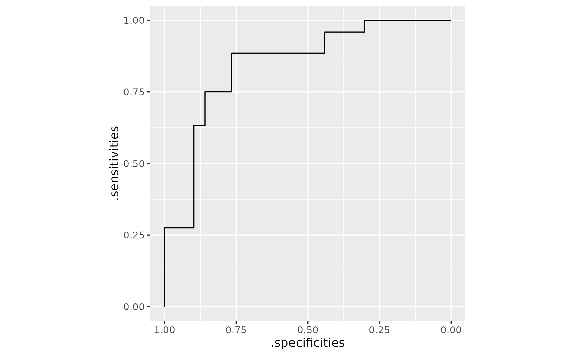
library(ggplot2)
# Plotting can be tricky bc sens and spec values repeat. geom_path() does the
# right thing and walks along threshold values to plot the sens-spec pairs
ggplot(roc_tbl) +
  aes(x = .specificities, y = .sensitivities) +
  geom_path() +
  scale_x_reverse() +
  coord_fixed(ratio = 1)