
A videogame speedrun is a challenge to beat the game as quickly as possible. It’s time attack racing but for a videogame. There are, in my mind, two ways to make a run’s time go faster: Playing better and more smoothly (optimizations, having better luck) and playing less of the game (better routing, new glitches/skips). The history of a speedrun category then is often an exciting mix of evolutionary improvements as players level up their skills and revolutionary jumps as players find new ways to cut through the game.
Summoning Salt is a Youtube creator who creates documentaries that trace out the world record progression in a speedrun. The videos are immensely enjoyable, as Salt dishes out the history bit by bit, record by record, sometimes in a suspenseful fashion.
As a data visualization person, I’ve noticed that Summoning Salt recently started to use a new prop in the videos: A step graph of the world record times. The graph is developed throughout a video as players (represented by individual colors) lower the times with new records (points) until you get a full reveal of a timeline like the following:
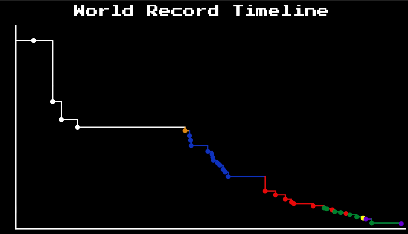
Let’s recreate this figure in R with ggplot2.
Warp pipe: Obtaining the data
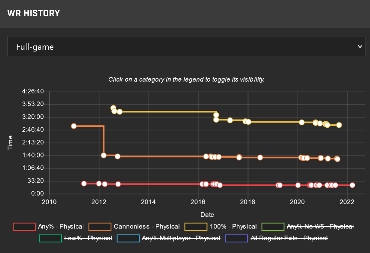
The game in question is New Super Mario Bros Wii, and the record keeper is the site speedrun.com. There is not just one speedrun category for this game, so in particular, we want the “Any%” record history (i.e., “any percent”: you don’t have play every level, and you can skip parts of the game.)
We need to get the leaderboard history data from speedrun.com. There is an official REST API for the site’s data, but it’s not straightforward how to query it to obtain the data needed for a world record progression. (Apparently, one could request the leaderboard on different dates and work backwards through time.) But that’s okay, we are not going to use the API. Instead, the statistics page for the game has a plot that is tantalizingly close to the one we want to create.
This plot is interactive, and our browser is downloading the data and plotting it for us. If we snoop around the page, we can find the JSON data behind the plot. In Firefox, when I right-click on the plot and hit “Inspect”, I see the HTML code that contains the plot. Just below the plot’s div is a chunk of Javascript.
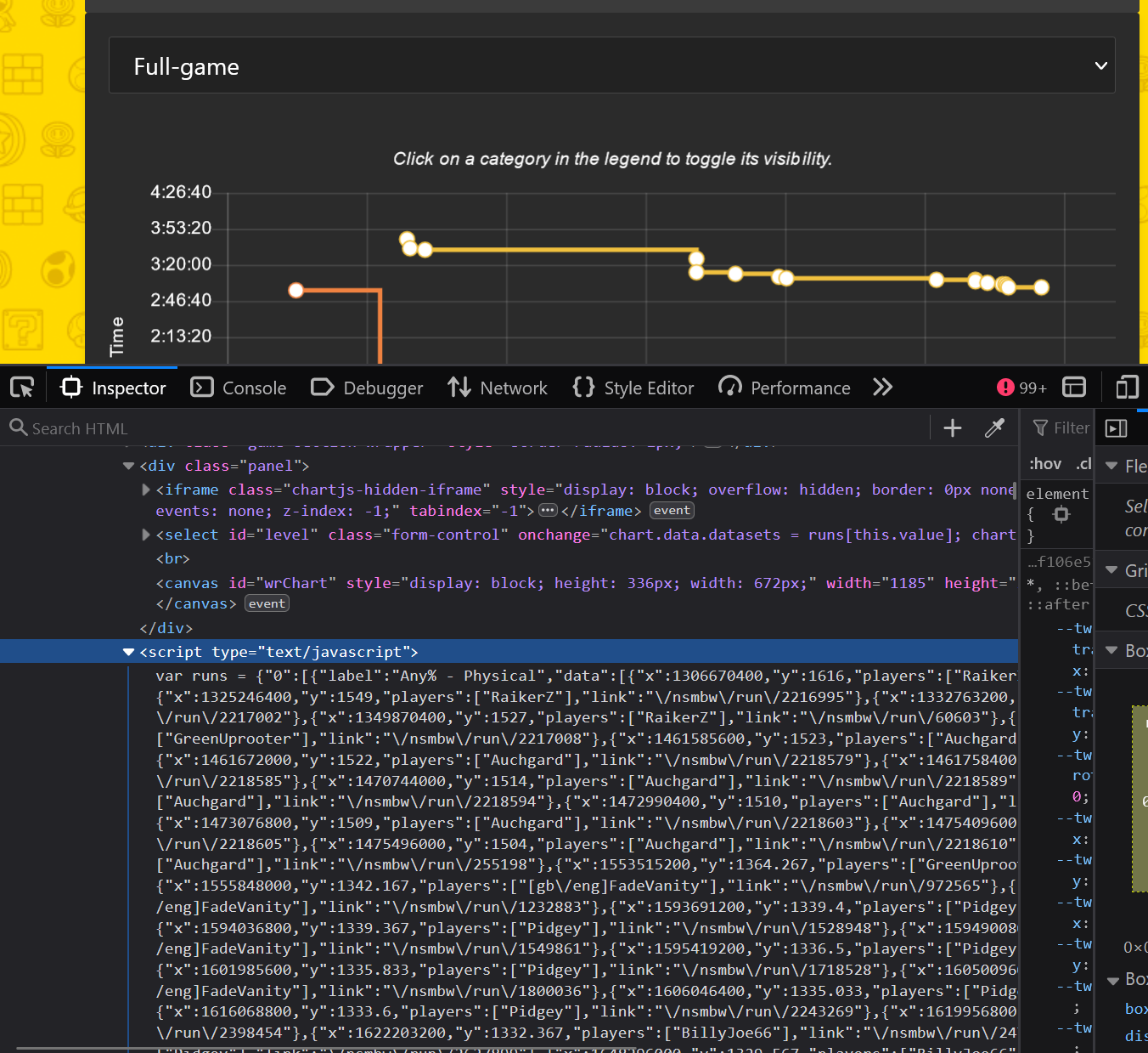
The first line of it is all the speedrun data that is being plotted. We save that JSON into its own file.
Ground pound: Filtering and cleaning the data
Let’s read the data into R. JSON is short for “Javascript Object
Notation”, and it’s basically the equivalent of a list() in R. Hence,
jsonlite provides a large, deeply nested list for us.
library(tidyverse)

# a helper function to download the data from github
# in case you want to play along
path_blog_data <- function(x) {
  file.path(
    "https://raw.githubusercontent.com",
    "tjmahr/tjmahr.github.io/master/_R/data",
    x
  )
}

json_runs <- path_blog_data("2022-05-23-nsmbw-runs.json") |>
  jsonlite::read_json()
The plot on the statistics page has a dropdown menu for different
kinds of records to display, so this JSON object has a sublist for each
dropdown menu choice. What we want is the first sublist (full game runs)
then its first sublist (with a label of "Any% - Physical") then its
"data".
# Dropdown menu choices
str(json_runs, max.level = 1)
#> List of 10
#>  $ 0   :List of 7
#>  $ 6789:List of 18
#>  $ 6805:List of 18
#>  $ 6815:List of 18
#>  $ 6826:List of 19
#>  $ 6841:List of 18
#>  $ 6846:List of 20
#>  $ 6859:List of 19
#>  $ 6868:List of 22
#>  $ 6882:List of 18

# Full game run histories
str(json_runs[[1]], max.level = 2)
#> List of 7
#>  $ :List of 7
#>   ..$ label                    : chr "Any% - Physical"
#>   ..$ data                     :List of 30
#>   ..$ borderColor              : chr "#EE4444"
#>   ..$ pointBorderColor         : chr "#EE4444"
#>   ..$ pointHoverBackgroundColor: chr "#EE4444"
#>   ..$ hidden                   : logi FALSE
#>   ..$ steppedLine              : logi TRUE
#>  $ :List of 7
#>   ..$ label                    : chr "Cannonless - Physical"
#>   ..$ data                     :List of 25
#>   ..$ borderColor              : chr "#EF8241"
#>   ..$ pointBorderColor         : chr "#EF8241"
#>   ..$ pointHoverBackgroundColor: chr "#EF8241"
#>   ..$ hidden                   : logi FALSE
#>   ..$ steppedLine              : logi TRUE
#>  $ :List of 7
#>   ..$ label                    : chr "100% - Physical"
#>   ..$ data                     :List of 17
#>   ..$ borderColor              : chr "#F0C03E"
#>   ..$ pointBorderColor         : chr "#F0C03E"
#>   ..$ pointHoverBackgroundColor: chr "#F0C03E"
#>   ..$ hidden                   : logi FALSE
#>   ..$ steppedLine              : logi TRUE
#>  $ :List of 7
#>   ..$ label                    : chr "Any% No W5 - Physical"
#>   ..$ data                     :List of 22
#>   ..$ borderColor              : chr "#8AC951"
#>   ..$ pointBorderColor         : chr "#8AC951"
#>   ..$ pointHoverBackgroundColor: chr "#8AC951"
#>   ..$ hidden                   : logi TRUE
#>   ..$ steppedLine              : logi TRUE
#>  $ :List of 7
#>   ..$ label                    : chr "Low% - Physical"
#>   ..$ data                     :List of 18
#>   ..$ borderColor              : chr "#09B876"
#>   ..$ pointBorderColor         : chr "#09B876"
#>   ..$ pointHoverBackgroundColor: chr "#09B876"
#>   ..$ hidden                   : logi TRUE
#>   ..$ steppedLine              : logi TRUE
#>  $ :List of 7
#>   ..$ label                    : chr "Any% Multiplayer - Physical"
#>   ..$ data                     :List of 11
#>   ..$ borderColor              : chr "#44BBEE"
#>   ..$ pointBorderColor         : chr "#44BBEE"
#>   ..$ pointHoverBackgroundColor: chr "#44BBEE"
#>   ..$ hidden                   : logi TRUE
#>   ..$ steppedLine              : logi TRUE
#>  $ :List of 7
#>   ..$ label                    : chr "All Regular Exits - Physical"
#>   ..$ data                     :List of 7
#>   ..$ borderColor              : chr "#6666EE"
#>   ..$ pointBorderColor         : chr "#6666EE"
#>   ..$ pointHoverBackgroundColor: chr "#6666EE"
#>   ..$ hidden                   : logi TRUE
#>   ..$ steppedLine              : logi TRUE

# Just want the data field from the first one
json_any_percent <- json_runs[[1]][[1]][["data"]]
Here are the first two points’ worth of date. We have a not-so-obviously
encoded date (x), the run length in seconds (y) and the player. We
are going to convert each of these lists into a dataframe and bind them
together.
json_any_percent |> head(2) |> str()
#> List of 2
#>  $ :List of 4
#>   ..$ x      : int 1306670400
#>   ..$ y      : int 1616
#>   ..$ players:List of 1
#>   .. ..$ : chr "RaikerZ"
#>   ..$ link   : chr "/nsmbw/run/2216987"
#>  $ :List of 4
#>   ..$ x      : int 1325246400
#>   ..$ y      : int 1549
#>   ..$ players:List of 1
#>   .. ..$ : chr "RaikerZ"
#>   ..$ link   : chr "/nsmbw/run/2216995"

data <- json_any_percent |>
  lapply(
    # turn one list into a dataframe
    function(x) {
      tibble(
        date = x$x,
        run_time_s = x$y,
        player = x$players[[1]]
      )
    }
  ) |>
  bind_rows()

data
#> # A tibble: 30 × 3
#>          date run_time_s player
#>         <int>      <dbl> <chr>
#>  1 1306670400       1616 RaikerZ
#>  2 1325246400       1549 RaikerZ
#>  3 1332763200       1531 RaikerZ
#>  4 1349870400       1527 RaikerZ
#>  5 1457179200       1526 GreenUprooter
#>  6 1461585600       1523 Auchgard
#>  7 1461672000       1522 Auchgard
#>  8 1461758400       1519 Auchgard
#>  9 1470744000       1514 Auchgard
#> 10 1471521600       1512 Auchgard
#> # … with 20 more rows
Lastly, we need to do something about those dates. When you see a date-time represented by a single large number, it’s probably a POSIX date representing the date-time as the number of seconds since some origin date-time (see also Unix Time). Using the default Unix origin time seems to give the correct date conversion:
data <- data |>
  mutate(
    date_posix = as.POSIXct(date, tz = "UTC", origin = "1970-01-01")
  )

data
#> # A tibble: 30 × 4
#>          date run_time_s player        date_posix
#>         <int>      <dbl> <chr>         <dttm>
#>  1 1306670400       1616 RaikerZ       2011-05-29 12:00:00
#>  2 1325246400       1549 RaikerZ       2011-12-30 12:00:00
#>  3 1332763200       1531 RaikerZ       2012-03-26 12:00:00
#>  4 1349870400       1527 RaikerZ       2012-10-10 12:00:00
#>  5 1457179200       1526 GreenUprooter 2016-03-05 12:00:00
#>  6 1461585600       1523 Auchgard      2016-04-25 12:00:00
#>  7 1461672000       1522 Auchgard      2016-04-26 12:00:00
#>  8 1461758400       1519 Auchgard      2016-04-27 12:00:00
#>  9 1470744000       1514 Auchgard      2016-08-09 12:00:00
#> 10 1471521600       1512 Auchgard      2016-08-18 12:00:00
#> # … with 20 more rows
Triple jump: Plotting
First, let’s get the data on the panel. I could spend an endless amount of time tweaking or customizing a plot’s theme, so I do the styling last. Otherwise, styling would fill up all of the time I’ve set aside to work on the plot.
We want to draw a point for each particular record-setting event, and we
want to draw a line that connects all of the points.
geom_step() draws a line plot but it can move
straight up/down or straight left/right—no diagonal lines—so it’s
what we want. We also want to the color of these geometries to change
with the record holder (player).
ggplot(data) +
  aes(x = date_posix, y = run_time_s, color = player) +
  geom_step() +
  geom_point()

Oops! It assumed that we wanted to connected the dots separately for
each color. We have to set the group aesthetic to a constant value so
there is only one line drawn.
ggplot(data) +
  aes(x = date_posix, y = run_time_s, color = player) +
  geom_step(aes(group = 1)) +
  geom_point()

Making the Summoning Salt version is just a matter of theming at this
point. We use theme_void() to completely wipe out
the current theme, and we hide the color legend.
ggplot(data) +
  aes(x = date_posix, y = run_time_s, color = player) +
  geom_step(aes(group = 1)) +
  geom_point() +
  theme_void() +
  guides(color = "none")

Next, we are going to use the showtext package to obtain an 8-bit font:
library(showtext)
#> Loading required package: sysfonts
#> Loading required package: showtextdb
font_add_google("Press Start 2P")
showtext_auto(TRUE)
The void theme provides nothing, so we have to specify the main colors, the axis lines, and the plotting margin. We also crank up the chroma values to have more intense colors for the black background.
ggplot(data) +
  aes(x = date_posix, y = run_time_s, color = player) +
  geom_step(aes(group = 1)) +
  geom_point() +
  guides(color = "none") +
  scale_color_discrete(c = 255) +
  labs(title = "World Record Timeline") +
  theme_void(base_size = 20, base_family = "Press Start 2P") +
  theme(
    plot.title = element_text(color = "white", hjust = .5),
    plot.background = element_rect(fill = "black"),
    axis.line = element_line(
      color = "white",
      size = 1,
      # more 8-bit looking lines
      lineend = "square"
    ),
    plot.margin = margin(12, 12, 12, 12, "pt")
  )

To keep overlapping points from looking like blobs, we can use a filled
point. For these, color is used on the border and fill is used on
the inside. We will set the outline of the points to black and the fill
to the player color. (If you look at more professional data
visualizations, you see this trick frequently with white bordering
around points.) With a new fill aesthetic in place, e have to make sure
that guide for the fill doesn’t appear and that fill and color have the
same color scale.
ggplot(data) +
  aes(x = date_posix, y = run_time_s, color = player) +
  geom_step(aes(group = 1)) +
  geom_point() +
  geom_point(
    aes(fill = player),
    shape = 21,
    color = "black",
    size = 2
  ) +
  # no legend for fill
  guides(color = "none", fill = "none") +
  # fill and color get same scale
  scale_color_discrete(c = 255, aesthetics = c("color", "fill")) +
  labs(title = "World Record Timeline") +
  theme_void(base_size = 20, base_family = "Press Start 2P") +
  theme(
    plot.title = element_text(color = "white", hjust = .5),
    plot.background = element_rect(fill = "black"),
    axis.line = element_line(
      color = "white",
      size = 1,
      lineend = "square"
    ),
    plot.margin = margin(12, 12, 12, 12, "pt")
  )

Finally, let’s make another version of this figure. How might we make a more accessible presentation of this information (of who held a record and when), assuming that we only have a static image? A legend with players/colors is a nonstarter. We could give each player their own distinct point shape so that color/shape encode the same information, but shapes get rough once you have to use more than four of them. We could use a player’s first letter instead of a point (show an F for FadeVanity) but the letters quickly overlap.
One idea would be to label the point with an annotation whenever there is a new record holder.
showtext_auto(FALSE)
data <- data |>
  mutate(
    # Remove the country flag annotation from this player
    player2 = ifelse(
      player == "[gb/eng]FadeVanity",
      "FadeVanity",
      player
    ),
    # Record whenever the title holder changes as an "era"
    change = player != lag(player) | is.na(lag(player)),
    era = cumsum(change)
  )

# I am going to hardcode some vertical position adjustments for the labels.
offsets <- c(1, 2, 1, 5, -1, 5, 4, 3, 2, 1, -4, -3, -2, -1)

data_lab <- data |>
  group_by(era) |>
  # Label the last point in an era
  filter(run_time_s == max(run_time_s)) |>
  ungroup() |>
  mutate(offset = offsets)

nudge_factor <- 30
ggplot(data) +
  aes(x = date_posix, y = run_time_s, color = player) +
  geom_text(
    aes(
      label = player2,
      y = run_time_s + nudge_factor * offset
    ),
    hjust = 0,
    size = 4,
    data = data_lab
  ) +
  geom_segment(
    aes(
      # i.e., run the line up to .95 of the label's nudging
      yend = run_time_s + nudge_factor * offset * .95,
      xend = date_posix
    ),
    data = data_lab,
    linetype = "dashed"
  ) +
  geom_step(aes(group = 1), size = 1) +
  geom_point(size = 3) +
  # yes, I'm adding forty million seconds to the last datetime
  expand_limits(x = max(data$date_posix) + 4e7) +
  guides(color = "none") +
  scale_x_datetime(
    name = NULL,
    date_breaks = "2 years",
    date_labels = "%Y"
  ) +
  scale_y_continuous(
    name = "World record",
    breaks = 21:27 * 60,
    # Show the minutes value with zero-padded seconds
    labels = function(x) sprintf("%d:%02.f", x %/% 60, x %% 60)
  ) +
  theme_minimal(base_size = 14) +
  theme(plot.margin = margin(12, 12, 12, 12, "pt"))

Last knitted on 2022-05-27. Source code on GitHub.1
-
.session_info
#> ─ Session info ───────────────────────────────────────────────────────────────
#>  setting  value
#>  version  R version 4.2.0 (2022-04-22 ucrt)
#>  os       Windows 10 x64 (build 22000)
#>  system   x86_64, mingw32
#>  ui       RTerm
#>  language (EN)
#>  collate  English_United States.utf8
#>  ctype    English_United States.utf8
#>  tz       America/Chicago
#>  date     2022-05-27
#>  pandoc   NA
#>
#> ─ Packages ───────────────────────────────────────────────────────────────────
#>  package     * version date (UTC) lib source
#>  assertthat    0.2.1   2019-03-21 [1] CRAN (R 4.2.0)
#>  backports     1.4.1   2021-12-13 [1] CRAN (R 4.2.0)
#>  broom         0.8.0   2022-04-13 [1] CRAN (R 4.2.0)
#>  cachem        1.0.6   2021-08-19 [1] CRAN (R 4.2.0)
#>  cellranger    1.1.0   2016-07-27 [1] CRAN (R 4.2.0)
#>  cli           3.3.0   2022-04-25 [1] CRAN (R 4.2.0)
#>  colorspace    2.0-3   2022-02-21 [1] CRAN (R 4.2.0)
#>  crayon        1.5.1   2022-03-26 [1] CRAN (R 4.2.0)
#>  curl          4.3.2   2021-06-23 [1] CRAN (R 4.2.0)
#>  DBI           1.1.2   2021-12-20 [1] CRAN (R 4.2.0)
#>  dbplyr        2.1.1   2021-04-06 [1] CRAN (R 4.2.0)
#>  digest        0.6.29  2021-12-01 [1] CRAN (R 4.2.0)
#>  downlit       0.4.0   2021-10-29 [1] CRAN (R 4.2.0)
#>  dplyr       * 1.0.9   2022-04-28 [1] CRAN (R 4.2.0)
#>  ellipsis      0.3.2   2021-04-29 [1] CRAN (R 4.2.0)
#>  evaluate      0.15    2022-02-18 [1] CRAN (R 4.2.0)
#>  fansi         1.0.3   2022-03-24 [1] CRAN (R 4.2.0)
#>  farver        2.1.0   2021-02-28 [1] CRAN (R 4.2.0)
#>  fastmap       1.1.0   2021-01-25 [1] CRAN (R 4.2.0)
#>  forcats     * 0.5.1   2021-01-27 [1] CRAN (R 4.2.0)
#>  fs            1.5.2   2021-12-08 [1] CRAN (R 4.2.0)
#>  generics      0.1.2   2022-01-31 [1] CRAN (R 4.2.0)
#>  ggplot2     * 3.3.6   2022-05-03 [1] CRAN (R 4.2.0)
#>  git2r         0.30.1  2022-03-16 [1] CRAN (R 4.2.0)
#>  glue          1.6.2   2022-02-24 [1] CRAN (R 4.2.0)
#>  gtable        0.3.0   2019-03-25 [1] CRAN (R 4.2.0)
#>  haven         2.5.0   2022-04-15 [1] CRAN (R 4.2.0)
#>  here          1.0.1   2020-12-13 [1] CRAN (R 4.2.0)
#>  highr         0.9     2021-04-16 [1] CRAN (R 4.2.0)
#>  hms           1.1.1   2021-09-26 [1] CRAN (R 4.2.0)
#>  httr          1.4.3   2022-05-04 [1] CRAN (R 4.2.0)
#>  jsonlite      1.8.0   2022-02-22 [1] CRAN (R 4.2.0)
#>  knitr       * 1.39    2022-04-26 [1] CRAN (R 4.2.0)
#>  labeling      0.4.2   2020-10-20 [1] CRAN (R 4.2.0)
#>  lifecycle     1.0.1   2021-09-24 [1] CRAN (R 4.2.0)
#>  lubridate     1.8.0   2021-10-07 [1] CRAN (R 4.2.0)
#>  magrittr      2.0.3   2022-03-30 [1] CRAN (R 4.2.0)
#>  memoise       2.0.1   2021-11-26 [1] CRAN (R 4.2.0)
#>  modelr        0.1.8   2020-05-19 [1] CRAN (R 4.2.0)
#>  munsell       0.5.0   2018-06-12 [1] CRAN (R 4.2.0)
#>  pillar        1.7.0   2022-02-01 [1] CRAN (R 4.2.0)
#>  pkgconfig     2.0.3   2019-09-22 [1] CRAN (R 4.2.0)
#>  purrr       * 0.3.4   2020-04-17 [1] CRAN (R 4.2.0)
#>  R6            2.5.1   2021-08-19 [1] CRAN (R 4.2.0)
#>  ragg          1.2.2   2022-02-21 [1] CRAN (R 4.2.0)
#>  readr       * 2.1.2   2022-01-30 [1] CRAN (R 4.2.0)
#>  readxl        1.4.0   2022-03-28 [1] CRAN (R 4.2.0)
#>  reprex        2.0.1   2021-08-05 [1] CRAN (R 4.2.0)
#>  rlang         1.0.2   2022-03-04 [1] CRAN (R 4.2.0)
#>  rprojroot     2.0.3   2022-04-02 [1] CRAN (R 4.2.0)
#>  rstudioapi    0.13    2020-11-12 [1] CRAN (R 4.2.0)
#>  rvest         1.0.2   2021-10-16 [1] CRAN (R 4.2.0)
#>  scales        1.2.0   2022-04-13 [1] CRAN (R 4.2.0)
#>  sessioninfo   1.2.2   2021-12-06 [1] CRAN (R 4.2.0)
#>  showtext    * 0.9-5   2022-02-09 [1] CRAN (R 4.2.0)
#>  showtextdb  * 3.0     2020-06-04 [1] CRAN (R 4.2.0)
#>  stringi       1.7.6   2021-11-29 [1] CRAN (R 4.2.0)
#>  stringr     * 1.4.0   2019-02-10 [1] CRAN (R 4.2.0)
#>  sysfonts    * 0.8.8   2022-03-13 [1] CRAN (R 4.2.0)
#>  systemfonts   1.0.4   2022-02-11 [1] CRAN (R 4.2.0)
#>  textshaping   0.3.6   2021-10-13 [1] CRAN (R 4.2.0)
#>  tibble      * 3.1.7   2022-05-03 [1] CRAN (R 4.2.0)
#>  tidyr       * 1.2.0   2022-02-01 [1] CRAN (R 4.2.0)
#>  tidyselect    1.1.2   2022-02-21 [1] CRAN (R 4.2.0)
#>  tidyverse   * 1.3.1   2021-04-15 [1] CRAN (R 4.2.0)
#>  tzdb          0.3.0   2022-03-28 [1] CRAN (R 4.2.0)
#>  utf8          1.2.2   2021-07-24 [1] CRAN (R 4.2.0)
#>  vctrs         0.4.1   2022-04-13 [1] CRAN (R 4.2.0)
#>  withr         2.5.0   2022-03-03 [1] CRAN (R 4.2.0)
#>  xfun          0.31    2022-05-10 [1] CRAN (R 4.2.0)
#>  xml2          1.3.3   2021-11-30 [1] CRAN (R 4.2.0)
#>  yaml          2.3.5   2022-02-21 [1] CRAN (R 4.2.0)
#>
#>  [1] C:/Users/Tristan/AppData/Local/R/win-library/4.2
#>  [2] C:/Program Files/R/R-4.2.0/library
#>
#> ──────────────────────────────────────────────────────────────────────────────
Leave a comment