Fitting a brms model with a stanli backend
This note is a stopgap demo of how to use a stanli backend with brms until the next version of brms (something newer than 2.23.0) comes out. (brms #1966 added an official stanli backend, and it was merged into the master branch of brms.)
Set up and install stanli:
install.packages("stanli", repos = c("https://seantalts.r-universe.dev"))
library(stanli)
stanli_install()
First, let’s fit a normal model with cmdstanr as a point of comparison for stanli’s performance gains.
The current demo of brms usage with stanli doesn’t feature priors or a custom model family, so we will use a contrived example with both:
library(stanli)
library(brms)
# stanli::stanli_install()

# Make a model from scratch
data <- lme4::sleepstudy
formula <- bf(
  Reaction ~ Days + (Days | Subject),
  # Just to test a non-default family
  family = student()
)

# Loose basis for some priors
lme4::sleepstudy$Reaction |> mean()
#> [1] 298.5079
lme4::sleepstudy$Reaction |> sd()
#> [1] 56.32876
rexp(1000, .01) |> fivenum()
#> [1]   0.04885372  30.38196331  70.14801274 145.45496673 768.92542630
rexp(1000, .10) |> fivenum()
#> [1]  0.01731279  3.01678405  6.65988896 13.43290706 72.51916389
rgamma(1000, .2, .01) |> fivenum()
#> [1] 1.535653e-14 7.973998e-02 2.084129e+00 1.617510e+01 2.501939e+02

priors <- prior(normal(300, 100), class = Intercept) +
  prior(normal(0, 100), class = b) +
  prior(exponential(0.01), class = sigma) +
  prior(exponential(0.01), class = sd, group = Subject, coef = Intercept) +
  prior(exponential(0.10), class = sd, group = Subject, coef = Days) +
  prior(lkj(2), class = cor)

check <- validate_prior(priors, formula, data)

model_cmdstanr <- brm(
  formula = formula,
  data = lme4::sleepstudy,
  prior = priors,
  backend = "cmdstanr",
  cores = 4,
  file = "2026-11-17-model1",
  file_refit = "on_change",
)

model_cmdstanr
#> Loading required namespace: rstan
#>  Family: student
#>   Links: mu = identity
#> Formula: Reaction ~ Days + (Days | Subject)
#>    Data: lme4::sleepstudy (Number of observations: 180)
#>   Draws: 4 chains, each with iter = 2000; warmup = 1000; thin = 1;
#>          total post-warmup draws = 4000
#>
#> Multilevel Hyperparameters:
#> ~Subject (Number of levels: 18)
#>                     Estimate Est.Error l-95% CI u-95% CI Rhat Bulk_ESS Tail_ESS
#> sd(Intercept)          32.11      6.91    21.21    48.30 1.00     1663     2165
#> sd(Days)                7.08      1.43     4.80    10.46 1.00     1742     2107
#> cor(Intercept,Days)    -0.05      0.24    -0.50     0.43 1.00     1335     1932
#>
#> Regression Coefficients:
#>           Estimate Est.Error l-95% CI u-95% CI Rhat Bulk_ESS Tail_ESS
#> Intercept   250.94      8.22   234.50   267.77 1.00     1353     1955
#> Days         10.72      1.79     7.20    14.20 1.00     1352     1804
#>
#> Further Distributional Parameters:
#>       Estimate Est.Error l-95% CI u-95% CI Rhat Bulk_ESS Tail_ESS
#> sigma    15.05      1.84    11.65    18.87 1.00     2632     2397
#> nu        3.36      1.12     1.90     6.19 1.00     3171     2484
#>
#> Draws were sampled using sample(hmc). For each parameter, Bulk_ESS
#> and Tail_ESS are effective sample size measures, and Rhat is the potential
#> scale reduction factor on split chains (at convergence, Rhat = 1).
stanli is going to run a Stan program for us, so we need to prepare the things that a Stan program needs (code and data). Then we define a model and sample from it:
scode <- stancode(object = formula, data = data, prior = priors)
sdata <- standata(object = formula, data = data, prior = priors)
model <- stanli_model(code = scode, data = sdata)
fit <- sample_model(model, chains = 4, refresh = 0)
Note that there was no compilation.
Now, the current trick is to tell brms to fit the model using a "mock"1
backend.
model_stanli <- brm(
  formula = formula,
  data = data,
  prior = priors,
  backend = "mock",
  mock_fit = as_stanfit(fit)
)
model_stanli
#>  Family: student
#>   Links: mu = identity
#> Formula: Reaction ~ Days + (Days | Subject)
#>    Data: data (Number of observations: 180)
#>   Draws: 4 chains, each with iter = 2000; warmup = 1000; thin = 1;
#>          total post-warmup draws = 4000
#>
#> Multilevel Hyperparameters:
#> ~Subject (Number of levels: 18)
#>                     Estimate Est.Error l-95% CI u-95% CI Rhat Bulk_ESS Tail_ESS
#> sd(Intercept)          31.93      6.87    20.96    47.22 1.00     1533     2203
#> sd(Days)                7.09      1.45     4.81    10.40 1.00     1611     2224
#> cor(Intercept,Days)    -0.07      0.24    -0.51     0.40 1.01     1268     1664
#>
#> Regression Coefficients:
#>           Estimate Est.Error l-95% CI u-95% CI Rhat Bulk_ESS Tail_ESS
#> Intercept   251.10      8.18   235.19   267.16 1.00     1381     1934
#> Days         10.73      1.83     7.05    14.28 1.00     1346     1791
#>
#> Further Distributional Parameters:
#>       Estimate Est.Error l-95% CI u-95% CI Rhat Bulk_ESS Tail_ESS
#> sigma    15.06      1.86    11.67    18.86 1.00     2243     2574
#> nu        3.38      1.11     1.88     6.18 1.00     3051     2666
#>
#> Draws were sampled using sampling(NUTS). For each parameter, Bulk_ESS
#> and Tail_ESS are effective sample size measures, and Rhat is the potential
#> scale reduction factor on split chains (at convergence, Rhat = 1).
This model should work like a regular brms model:
pp_check(model_stanli)
#> Using 10 posterior draws for ppc type 'dens_overlay' by default.
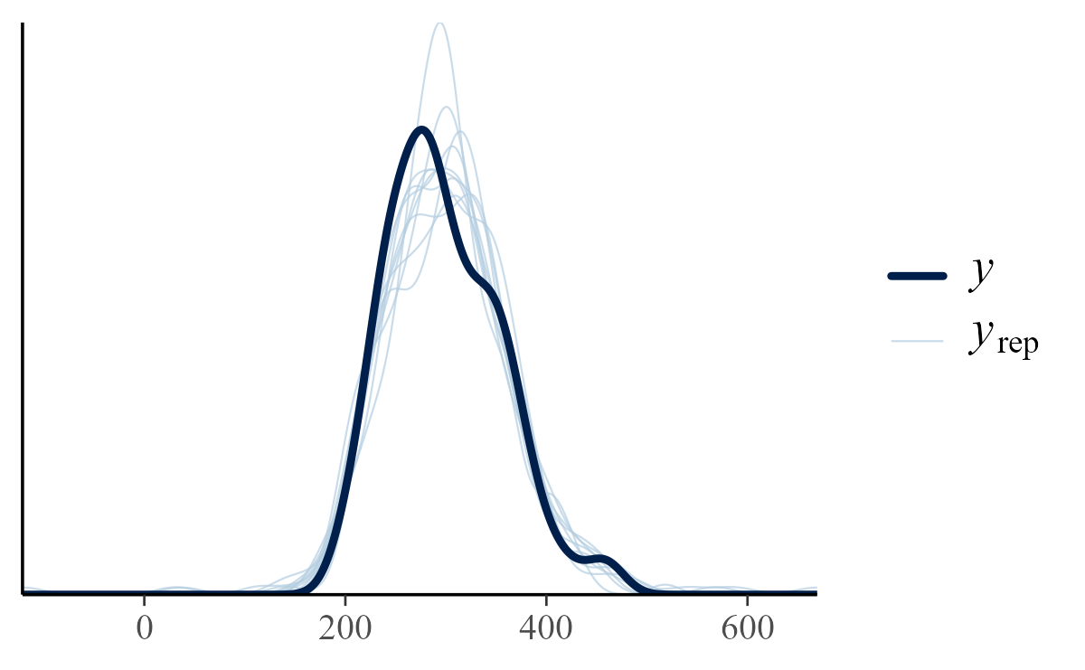
Posterior predictive density
If we already have a brms-fitted version of the model around, we skip the data
and code steps and use update.brmsfit() instead:
model_stanli2 <- update(
  model_cmdstanr,
  backend = "mock",
  mock_fit = as_stanfit(fit),
  recompile = TRUE
)
model_stanli2
#>  Family: student
#>   Links: mu = identity
#> Formula: Reaction ~ Days + (Days | Subject)
#>    Data: lme4::sleepstudy (Number of observations: 180)
#>   Draws: 4 chains, each with iter = 2000; warmup = 1000; thin = 1;
#>          total post-warmup draws = 4000
#>
#> Multilevel Hyperparameters:
#> ~Subject (Number of levels: 18)
#>                     Estimate Est.Error l-95% CI u-95% CI Rhat Bulk_ESS Tail_ESS
#> sd(Intercept)          31.93      6.87    20.96    47.22 1.00     1533     2203
#> sd(Days)                7.09      1.45     4.81    10.40 1.00     1611     2224
#> cor(Intercept,Days)    -0.07      0.24    -0.51     0.40 1.01     1268     1664
#>
#> Regression Coefficients:
#>           Estimate Est.Error l-95% CI u-95% CI Rhat Bulk_ESS Tail_ESS
#> Intercept   251.10      8.18   235.19   267.16 1.00     1381     1934
#> Days         10.73      1.83     7.05    14.28 1.00     1346     1791
#>
#> Further Distributional Parameters:
#>       Estimate Est.Error l-95% CI u-95% CI Rhat Bulk_ESS Tail_ESS
#> sigma    15.06      1.86    11.67    18.86 1.00     2243     2574
#> nu        3.38      1.11     1.88     6.18 1.00     3051     2666
#>
#> Draws were sampled using sampling(NUTS). For each parameter, Bulk_ESS
#> and Tail_ESS are effective sample size measures, and Rhat is the potential
#> scale reduction factor on split chains (at convergence, Rhat = 1).
We can compare sampling performance. This is a pretty fast model to begin with, so the gains here might be more limited compared to a more complex model.
rstan::get_elapsed_time(model_cmdstanr$fit)
#>         warmup sample
#> chain:1  2.117  0.981
#> chain:2  2.009  1.047
#> chain:3  1.897  1.030
#> chain:4  2.232  1.031

rstan::get_elapsed_time(model_stanli$fit)
#>            warmup    sample
#> chain:1 0.6565742 0.2930656
#> chain:2 0.6128654 0.2871662
#> chain:3 0.6307627 0.2910862
#> chain:4 0.5246784 0.2682132

# If we want to say "n-times faster"
rstan::get_elapsed_time(model_cmdstanr$fit) /
  rstan::get_elapsed_time(model_stanli$fit)
#>           warmup   sample
#> chain:1 3.224312 3.347373
#> chain:2 3.278044 3.645972
#> chain:3 3.007470 3.538471
#> chain:4 4.254034 3.843957
But don’t forget compile time:
stan_file <- tempfile(fileext = ".stan")
writeLines(scode, stan_file)

compile_time <- system.time({
  model <- cmdstanr::cmdstan_model(
    stan_file,
    force_recompile = TRUE
  )
})
compile_time
#>    user  system elapsed
#>    0.09    0.06   23.87

cmdstanr_total <- model_cmdstanr$fit |>
  rstan::get_elapsed_time() |>
  rowSums() |>
  max()

stanli_total <- model_stanli$fit |>
  rstan::get_elapsed_time() |>
  rowSums() |>
  max()

(cmdstanr_total + unname(compile_time[3])) / stanli_total
#> [1] 28.57189
-
In software testing, we might define a “mock” version of a computation, like a file download, where we skip the actual and maybe unpredictable work and load up a prepared result. brms can test model preparation by skipping model compilation and skipping sampling with a mock backend and loading in some prepared MCMC samples. That’s how we can understand what this code is doing. ↩
Leave a comment