Confidence interval overlap and p-values
Two 95% confidence intervals can overlap and still have a statistically significant difference at p = .05. I want to refresh my memory on what p-values are implied by different degrees of overlap and simulate the rules of thumb myself.
Cumming (2008) provides a summary of some visual rules of thumb. (This is the same author of 2014 The New Statistics manifesto.) Here are the main points I wanted to recall:
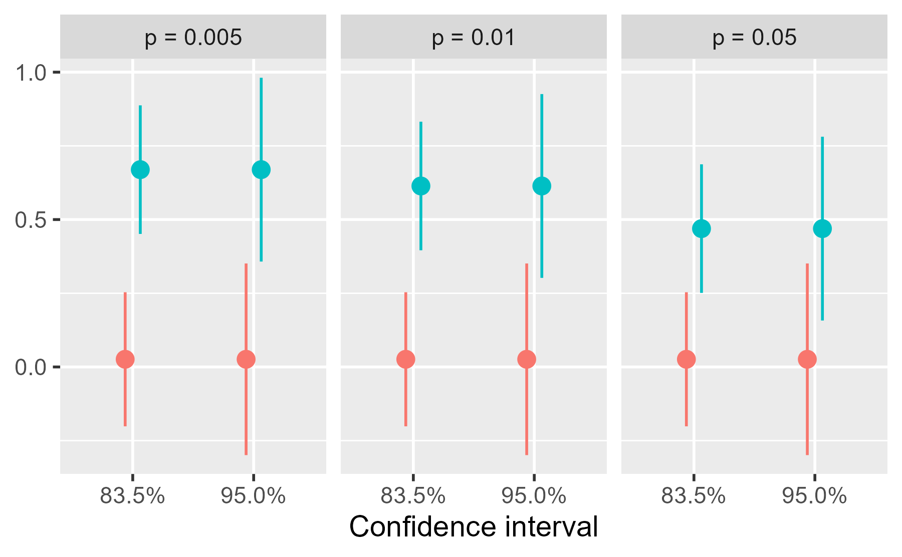
- Two 95% intervals can overlap by a small amount at p = .01.
- Two 83.5% intervals will just touch at p = .05.
- Two 95% intervals can overlap up to half the length of an interval whisker at p = .05.
We simulate data sets that yield a target p-value.
simulate_group_data_for_given_p_value <- function(
    p_target,
    n_a = 40,
    n_b = NULL,
    sd_a = 1,
    sd_b = NULL,
    seed = NULL
) {
  if (!is.null(seed)) withr::local_seed(seed)
  n_b <- n_b %||% n_a
  sd_b <- sd_b %||% sd_a
  data_a <- rnorm(n_a, 0, sd_a)
  data_b <- rnorm(n_b, 0, sd_b)

  get_p_val <- function(diff) t.test(data_a, data_b + diff)[["p.value"]]

  target_diff <- uniroot(
    f = function(x) get_p_val(x) - p_target,
    interval = c(0, 5 * sd_a),
    tol = p_target / 1000,
    extendInt = "yes"
  )
  data.frame(
    group = c(rep("a", n_a), rep("b", n_b)),
    value = c(data_a, data_b + target_diff$root),
    target_p_value = paste0("p = ", p_target)
  )
}
Test the data simulation functions.
data1 <- simulate_group_data_for_given_p_value(.05, seed = 20250723)
t.test(value ~ group, data1) |>
  broom::tidy() |>
  str()
#> tibble [1 × 10] (S3: tbl_df/tbl/data.frame)
#>  $ estimate   : num -0.443
#>  $ estimate1  : num 0.026
#>  $ estimate2  : num 0.469
#>  $ statistic  : Named num -1.99
#>   ..- attr(*, "names")= chr "t"
#>  $ p.value    : num 0.05
#>  $ parameter  : Named num 77.9
#>   ..- attr(*, "names")= chr "df"
#>  $ conf.low   : num -0.887
#>  $ conf.high  : num -8.44e-07
#>  $ method     : chr "Welch Two Sample t-test"
#>  $ alternative: chr "two.sided"

data2 <- simulate_group_data_for_given_p_value(.01, seed = 20250723)
t.test(value ~ group, data2) |>
  broom::tidy() |>
  str()
#> tibble [1 × 10] (S3: tbl_df/tbl/data.frame)
#>  $ estimate   : num -0.588
#>  $ estimate1  : num 0.026
#>  $ estimate2  : num 0.614
#>  $ statistic  : Named num -2.64
#>   ..- attr(*, "names")= chr "t"
#>  $ p.value    : num 0.01
#>  $ parameter  : Named num 77.9
#>   ..- attr(*, "names")= chr "df"
#>  $ conf.low   : num -1.03
#>  $ conf.high  : num -0.145
#>  $ method     : chr "Welch Two Sample t-test"
#>  $ alternative: chr "two.sided"
Create a grid of CIs and plot them. Hmisc::smean.cl.normal() is used by
ggplot2 to compute the CI, and this function “the sample mean and
lower and upper Gaussian confidence limits based on the
t-distribution”.
library(tidyverse)
#> Warning: package 'tibble' was built under R version 4.5.2
#> Warning: package 'tidyr' was built under R version 4.5.2
#> Warning: package 'readr' was built under R version 4.5.2
#> Warning: package 'purrr' was built under R version 4.5.2
#> Warning: package 'dplyr' was built under R version 4.5.2
#> Warning: package 'stringr' was built under R version 4.5.2
#> Warning: package 'lubridate' was built under R version 4.5.2
#> ── Attaching core tidyverse packages ──────────────────────── tidyverse 2.0.0 ──
#> ✔ dplyr     1.2.0     ✔ readr     2.2.0
#> ✔ forcats   1.0.1     ✔ stringr   1.6.0
#> ✔ ggplot2   4.0.2     ✔ tibble    3.3.1
#> ✔ lubridate 1.9.5     ✔ tidyr     1.3.2
#> ✔ purrr     1.2.1
#> ── Conflicts ────────────────────────────────────────── tidyverse_conflicts() ──
#> ✖ dplyr::filter() masks stats::filter()
#> ✖ dplyr::lag()    masks stats::lag()
#> ℹ Use the conflicted package (<http://conflicted.r-lib.org/>) to force all conflicts to become errors
mean_ci <- function(x, width) {
  df <- ggplot2::mean_cl_normal(x, conf.int = width)
  df[[".width"]] <- width
  df
}

data <- bind_rows(
  data1,
  data2,
   simulate_group_data_for_given_p_value(.005, seed = 20250723)
)

cis <- data |>
  group_by(group, target_p_value) |>
  reframe(
    ci = list(mean_ci(value, .95), mean_ci(value, .835))
  ) |>
  tidyr::unnest(cols = ci)

ggplot(cis) +
  aes(x = factor(.width), color = group) +
  geom_pointrange(
    aes(ymin = ymin, y = y, ymax = ymax),
    position = position_dodge(width = .25)
  ) +
  facet_wrap(~target_p_value) +
  guides(color = "none") +
  scale_x_discrete(
    "Confidence interval",
    labels = function(x) scales::label_percent(.1)(as.numeric(x))
  ) +
  labs(y = NULL) +
  theme_grey(base_size = 14)
center
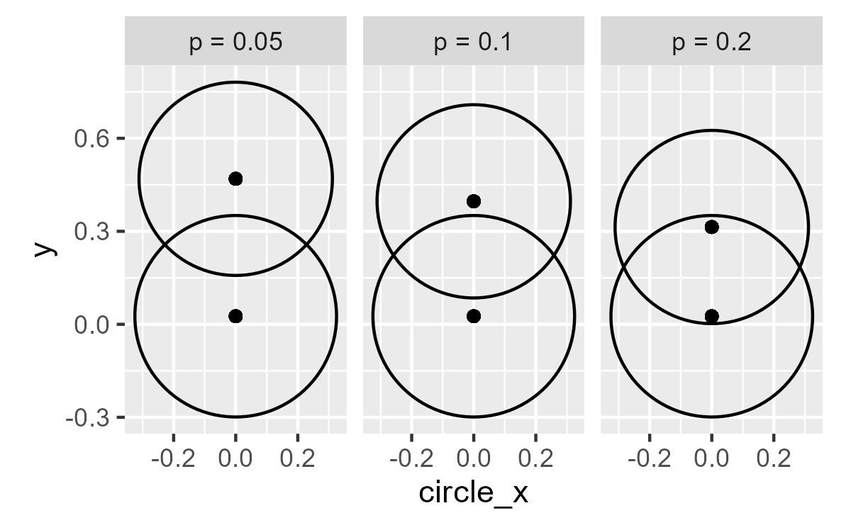
I was also intrigued by the following remark:
Sall [28] described an ingenious variation of overlap: Around any mean, draw a circle with radius equal to the margin of error of the 95 per cent CI. Sall showed that if two such circles overlap so that they intersect at right angles, p = 0.05 for the comparison of the two means.
So, when p = .05, the tangents at the intersections are right angles (?).
data_circles <- data1 |>
  bind_rows(
    simulate_group_data_for_given_p_value(.10, seed = 20250723),
    simulate_group_data_for_given_p_value(.20, seed = 20250723)
  ) |>
  group_by(group, target_p_value) |>
  reframe(
    ci = mean_ci(value, .95)
  ) |>
  tidyr::unnest(cols = ci) |>
  filter(.width == .95) |>
  mutate(
    radius = (ymax - ymin) / 2
  ) |>
  rowwise() |>
  mutate(
    angle = list(seq(0, 2 * pi, length.out = 100))
  ) |>
  ungroup() |>
  tidyr::unnest(cols = angle) |>
  mutate(
    circle_x = cos(angle) * radius,
    circle_y = y + sin(angle) * radius
  )

ggplot(data_circles) +
  geom_point(aes(x = 0, y = y)) +
  geom_path(aes(group = y, x = circle_x, y = circle_y)) +
  facet_wrap(~target_p_value) +
  coord_fixed()
center
Leave a comment