Computing the mean of the logit-normal with Stan’s integrate_1d()
Here is a quick note on using Stan to compute a 1-dimension integral.
Suppose we have a multilevel logistic regression model with a population mean of x logits and the random intercepts of the participants have an SD of s logits. What is the population average on the outcome scale (probabilities/proportions)?
In this situation, we have a logit-normal distribution. That is, the participant means are probabilities/proportions between 0 and 1, but on the logit scale, the participant means follow a Normal(x, s) distribution. There is no neat (closed-form) formula for computing the population average for given x and s values. We just have to average over that normal distribution somehow.
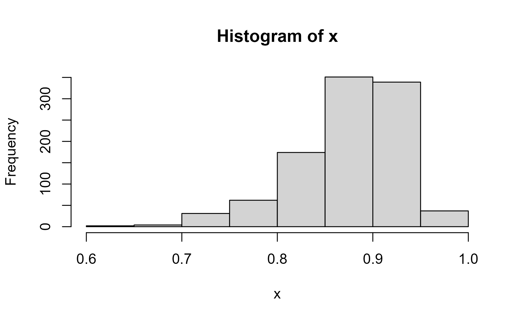
Let x = 2 and s = .5. We can simulate new participants, convert from logits to proportions and average. That option is always available to us, and it makes sense. We compute a population mean by making a population (large sample of simulated individuals) and averaging them together.
set.seed(20250708)
x <- rnorm(1000, 2, .5) |> plogis()
hist(x)
center
mean(x)
#> [1] 0.8745648
Rather than taking a random set of values, we can take 1000 quantiles along the normal distribution for a grid approximation.
# Get 1000 evenly spaced percentiles
ppoints(1000) |> qnorm(2, .5) |> plogis() |> mean()
#> [1] 0.8710035
Or we can do what the logitnorm package does and compute the actual integral.
logitnorm::momentsLogitnorm(2, .5)
#>        mean         var
#> 0.870993464 0.003167158
What’s nice about this integral is that it reads like a weighted average:
proportions provided by plogis() are weighted by the probability
density function dnorm().
logitnorm::momentsLogitnorm
#> function (mu, sigma, abs.tol = 0, ...)
#> {
#>     fExp <- function(x) plogis(x) * dnorm(x, mean = mu, sd = sigma)
#>     .exp <- integrate(fExp, -Inf, Inf, abs.tol = abs.tol, ...)$value
#>     fVar <- function(x) (plogis(x) - .exp)^2 * dnorm(x, mean = mu,
#>         sd = sigma)
#>     .var <- integrate(fVar, -Inf, Inf, abs.tol = abs.tol, ...)$value
#>     c(mean = .exp, var = .var)
#> }
#> <bytecode: 0x0000026093c02148>
#> <environment: namespace:logitnorm>
#> attr(,"ex")
#> function ()
#> {
#>     (res <- momentsLogitnorm(4, 1))
#>     (res <- momentsLogitnorm(5, 0.1))
#> }
#> <environment: namespace:logitnorm>
(Note that logitnorm also computes the variance, so its source code has two
integrals. We care about the fExp() function. Note also the neat idea of
attaching function examples to the function as an attribute.)
In my experience, where I wanted to compute a population average on each draw of a posterior interval or for each row of a dataframe, I wrote a vectorized wrapper over logitnorm so we can compute means from vectors of means or sigmas:
wisclabmisc::logitnorm_mean(2, .5)
#>      mean
#> 0.8709935

wisclabmisc::logitnorm_mean(c(1, 2, 3), .5)
#> [1] 0.7205808 0.8709935 0.9473300
For fun, we could have Stan compute this integral for us. We have to
follow a specific recipe. We first have to define the integrand, which
would be the weighted outcome for a specific logit value. This integrand
function needs to follow a specific convention in order to be passed to
integrate_1d() later.
The next block shows the simple form of the function and the form of the function suitable for integration:
// this is Stan code
functions {
  // Nice version of the integrand function
  real inv_logit_times_normal(real x, real mu, real sigma) {
    real log_phi = normal_lpdf(x | mu, sigma);
    return inv_logit(x) * exp(log_phi);
  }

  // Generic version of function suitable for passing to integrate_1d()
  real integrand_inv_logit_times_normal(
      real x,                  // variable we integrate over
      real xc,
      array[] real theta,      // parameters for the integral
      data array[] real x_r,
      data array[] int x_i
  ) {
    real mu = theta[1];
    real sigma = theta[2];
    // Stan's normal_lpdf is like R's dnorm(log = TRUE) so we exp() it
    real log_phi = normal_lpdf(x | mu, sigma);
    return inv_logit(x) * exp(log_phi);
  }
}
The two important parameters mu and sigma from the first function
get stuffed into an array theta in the second version of the function.
There are also additional standard arguments to the second version of
the function. They seem to help integration (xc) or provide a way to
pass data/transformed data into the function (x_r, x_i). Based
on error messages I’ve gotten—
  [...]
  The 5th argument must be data-only. (Local variables are assumed to depend
  on parameters; same goes for function inputs unless they are marked with
  the keyword 'data'.)
—I assume that we need a clean route for data to enter the functions
so that the code analysis knows what depends on parameters (versus what
depends on data), and x_r and x_i provide that route. But that’s
just my speculation!
Now we can make the functions that compute the integral with
integrate_1d() for a given mu and sigma. integrate_1d() seems
pretty straightforward as we tell it the function to integrate
over, the limits of integration and provide the parameter array theta.
In the last two arguments, we provide zero-filled arrays for x_r and x_i
so that those mandatory but unused function arguments have values.
I also defined a vectorized version of the function after I got the simple version working.
// this is Stan code
functions {
  // functions from above omitted
  // [...]

  // Compute the integral
  real logitnormal_mean(real mu, real sigma) {
    return integrate_1d(
      integrand_inv_logit_times_normal,
      negative_infinity(),
      positive_infinity(),
      {mu, sigma},
      {0.0},
      {0}
    );
  }


  // Vectorized version
  vector logitnormal_mean2(vector mu, vector sigma) {
    int N = num_elements(mu);
    vector[N] result;

    for (n in 1:N) {
      result[n] = integrate_1d(
        integrand_inv_logit_times_normal,
        negative_infinity(),
        positive_infinity(),
        {mu[n], sigma[n]},
        {0.0},
        {0}
      );
    }
    return result;
  }
}
Here is how we would get Stan to compile these functions and provide them to use in R.
model_code <- '
functions {
  // Nice version of the integrand function
  real inv_logit_times_normal(real x, real mu, real sigma) {
    real log_phi = normal_lpdf(x | mu, sigma);
    return inv_logit(x) * exp(log_phi);
  }

  // Generic version of function suitable for passing to integrate_1d
  real integrand_inv_logit_times_normal(
      real x,                  // variable we integrate over
      real xc,
      array[] real theta,      // parameters for the integral
      data array[] real x_r,
      data array[] int x_i
  ) {
    real mu = theta[1];
    real sigma = theta[2];
    real log_phi = normal_lpdf(x | mu, sigma);
    return inv_logit(x) * exp(log_phi);
  }

  // Compute the integral
  real logitnormal_mean(real mu, real sigma) {
    return integrate_1d(
      integrand_inv_logit_times_normal,
      negative_infinity(),
      positive_infinity(),
      {mu, sigma},
      {0.0},
      {0}
    );
  }


  // Vectorized version
  vector logitnormal_mean2(vector mu, vector sigma) {
    int N = num_elements(mu);
    vector[N] result;

    for (n in 1:N) {
      result[n] = integrate_1d(
        integrand_inv_logit_times_normal,
        negative_infinity(),
        positive_infinity(),
        {mu[n], sigma[n]},
        {0.0},
        {0}
      );
    }
    return result;
  }
}
'

m <- cmdstanr::cmdstan_model(
  cmdstanr::write_stan_file(model_code),
  exe_file = "logit-demo.exe",
  compile = FALSE
)
m$compile(compile_standalone = TRUE)
#> In file included from stan/src/stan/model/model_header.hpp:5:
#> stan/src/stan/model/model_base_crtp.hpp:205:8: warning: 'void stan::model::model_base_crtp<M>::write_array(stan::rng_t&, std::vector<double>&, std::vector<int>&, std::vector<double>&, bool, bool, std::ostream*) const [with M = model_757f8c23c1c462e2a00abaf4bc9c7c82_model_namespace::model_757f8c23c1c462e2a00abaf4bc9c7c82_model; stan::rng_t = boost::random::mixmax_engine<17, 36, 0>; std::ostream = std::basic_ostream<char>]' was hidden [-Woverloaded-virtual=]
#>   205 |   void write_array(stan::rng_t& rng, std::vector<double>& theta,
#>       |        ^~~~~~~~~~~
#> C:/Users/Tristan/AppData/Local/Temp/RtmpEP1vp4/model-4ea829e277e4.hpp:457: note:   by 'model_757f8c23c1c462e2a00abaf4bc9c7c82_model_namespace::model_757f8c23c1c462e2a00abaf4bc9c7c82_model::write_array'
#>   457 |   write_array(RNG& base_rng, std::vector<double>& params_r, std::vector<int>&
#> stan/src/stan/model/model_base_crtp.hpp:136:8: warning: 'void stan::model::model_base_crtp<M>::write_array(stan::rng_t&, Eigen::VectorXd&, Eigen::VectorXd&, bool, bool, std::ostream*) const [with M = model_757f8c23c1c462e2a00abaf4bc9c7c82_model_namespace::model_757f8c23c1c462e2a00abaf4bc9c7c82_model; stan::rng_t = boost::random::mixmax_engine<17, 36, 0>; Eigen::VectorXd = Eigen::Matrix<double, -1, 1>; std::ostream = std::basic_ostream<char>]' was hidden [-Woverloaded-virtual=]
#>   136 |   void write_array(stan::rng_t& rng, Eigen::VectorXd& theta,
#>       |        ^~~~~~~~~~~
#> C:/Users/Tristan/AppData/Local/Temp/RtmpEP1vp4/model-4ea829e277e4.hpp:457: note:   by 'model_757f8c23c1c462e2a00abaf4bc9c7c82_model_namespace::model_757f8c23c1c462e2a00abaf4bc9c7c82_model::write_array'
#>   457 |   write_array(RNG& base_rng, std::vector<double>& params_r, std::vector<int>&
compile_standalone will tell Stan to compile and “expose” the
functions so that R can call them.
Now we can access the function and get the marginal mean:
m$functions$logitnormal_mean(mu = 2, sigma = .5)
#> [1] 0.8709935
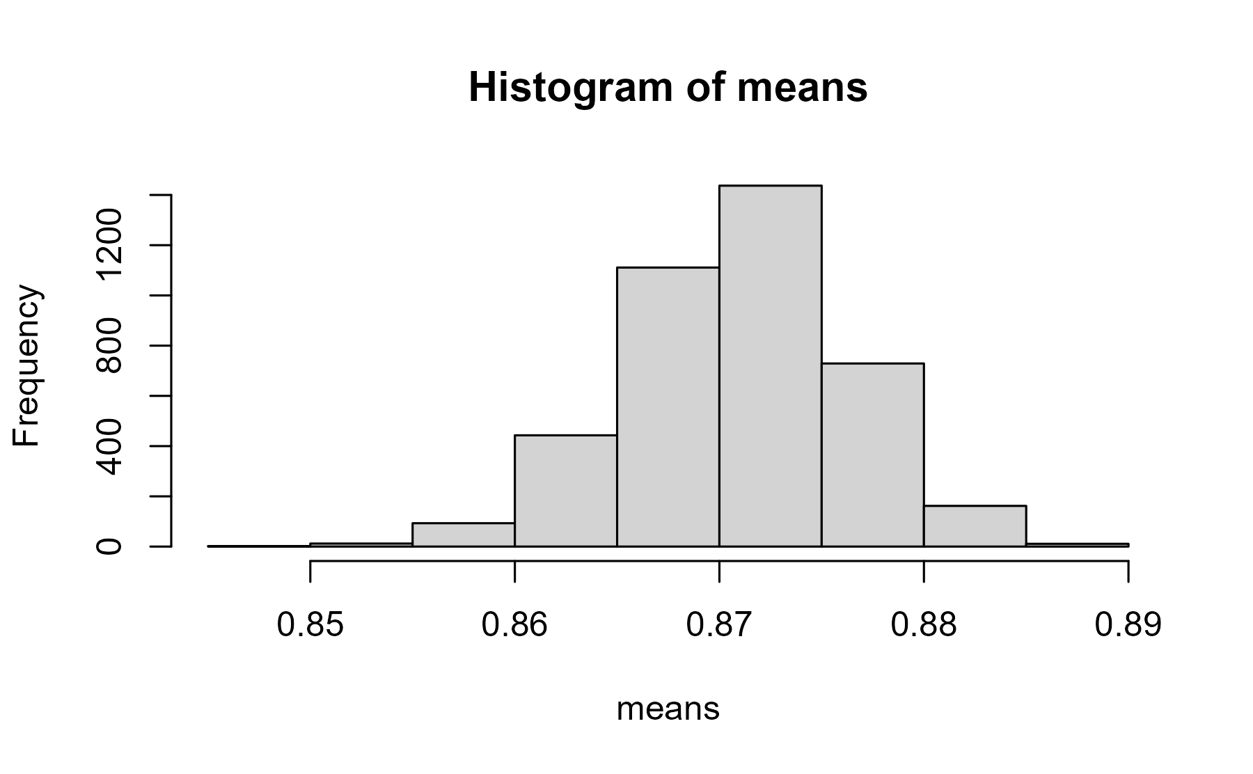
Or if say we have a posterior distribution of them we might try the vectorized version:
mus <- 2 + rnorm(4000, 0, .05)
sigmas <- .5 + rnorm(4000, 0, .01)

means <- m$functions$logitnormal_mean2(
  mu = mus,
  sigma = sigmas
)
hist(means)
center
# Check against logitnorm implementation
means2 <- wisclabmisc::logitnorm_mean(mus, sigmas)
all.equal(means, means2)
#> [1] TRUE
In an actual model, it would probably be smarter to compute this integral in the
generated quantities block so that this marginal mean becomes available
like any other posterior variable.
Quick benchmark:
microbenchmark::microbenchmark(
  m$functions$logitnormal_mean2(mu = mus, sigma = sigmas),
  wisclabmisc::logitnorm_mean(mus, sigmas),
  times = 20
)
#> Unit: milliseconds
#>                                                     expr       min        lq
#>  m$functions$logitnormal_mean2(mu = mus, sigma = sigmas)  116.1777  116.3773
#>                 wisclabmisc::logitnorm_mean(mus, sigmas) 1131.4982 1135.8255
#>       mean    median        uq       max neval
#>   125.0364  116.7694  117.7948  195.5061    20
#>  1163.6127 1141.8094 1159.8912 1405.3907    20
Leave a comment