
I recently developed and released an R package called
solarizeddocx. It provides solarizeddocx::document(), an
RMarkdown output format for
solarized-highlighted Microsoft Word documents . The image below
shows a comparison of the solarizeddocx and the default docx format:
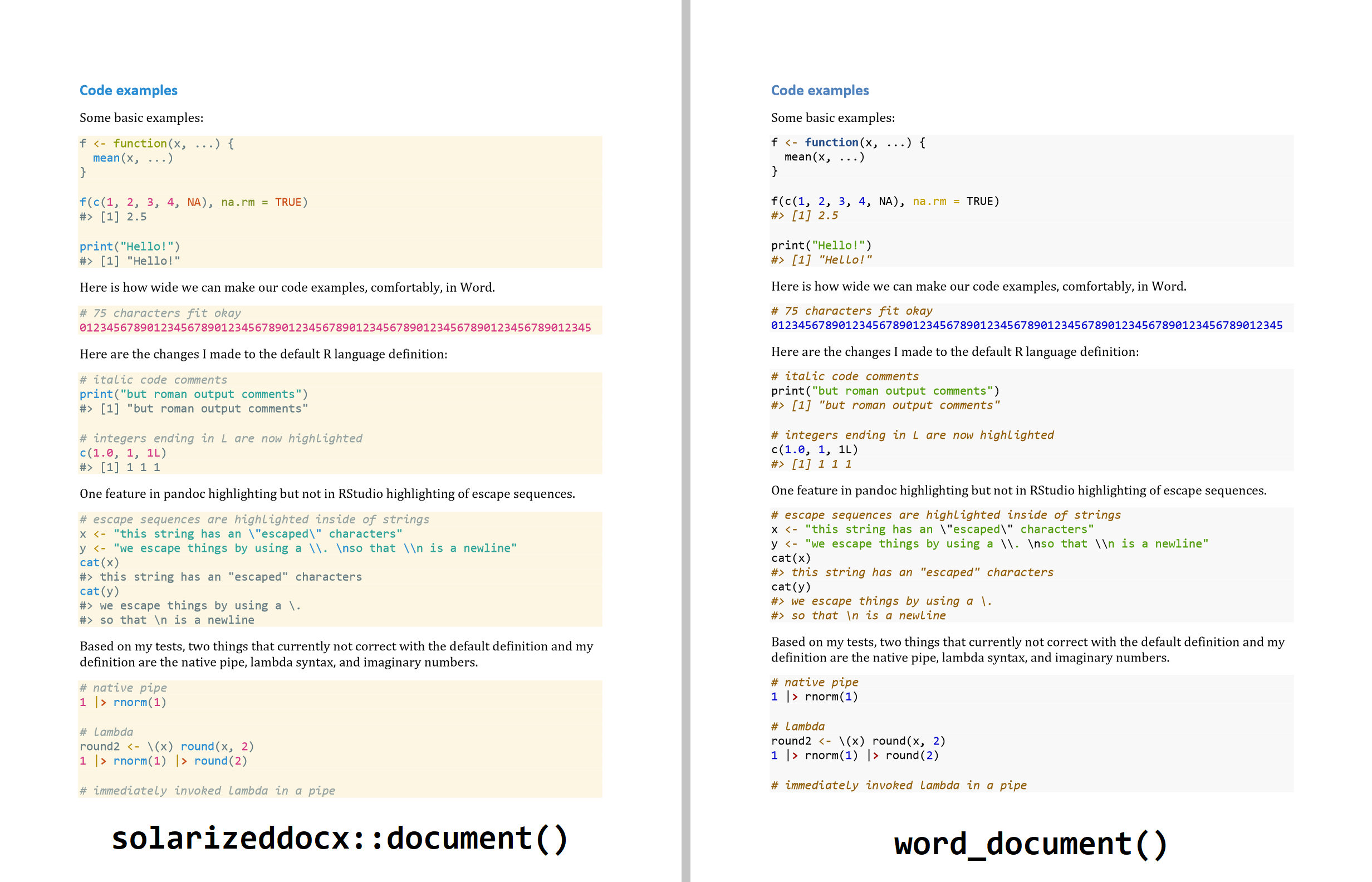
solarizeddocx::document() and rmarkdown::word_document().
The package provides a demo document which is essentially a vignette where I describe all the customizations used by the package and put the syntax highlighting to the test. The demo can be rendered and viewed with:
# install.packages("devtools")
devtools::install_github("tjmahr/solarizeddocx")
solarizeddocx::demo_document()
The format can used in RMarkdown document via YAML metadata.
output:
  solarizeddocx::document: default
Or explicitly with rmarkdown:
rmarkdown::render(
  "README.Rmd",
  output_format = solarizeddocx::document()
)
solarizeddocx also exports its document assets so that they can be used in other output formats, and it exports theme-building tools to create new pandoc syntax highlighting themes. I am most proud of these features, so I will demonstrate each of these in turn and create a brand new syntax highlighting theme in this post.
knitr: .Rmd to .md conversion
To give a simplified description, RMarkdown works by knitting the code in an RMarkdown (.Rmd) file with knitr to obtain a markdown (.md) file and then post-processing this knitr output with other tools. In particular, it uses pandoc which converts between all kinds of document formats. For this demonstration, we will do the knitting and pandoc steps separately without relying on RMarkdown. That said, the options we pass to pandoc can usually be used in RMarkdown (as we demonstrate at the very end of this post).
Our input file is a small .Rmd file. It’s very basic, meant to illustrate some function calls, strings, numbers, code comments and output.
```{r, include = FALSE}
knitr::opts_chunk$set(collapse = TRUE, comment = "#>")
```
Fit a model with `lm`():
```{r}
model <- lm(mpg ~ 1 + cyl, mtcars)
coefs <- coef(model)

# prediction for 8 cylinders
coefs["(Intercept)"] + 8 * coefs["cyl"]

predict(model, data.frame(cyl = 8L))
```
We knit() the document to run the code and store results
in a markdown file. (Actually, we use knit_child()
because I was getting some weird using-knit()-inside-of-knit()
issues when rendering this post. But in general, we would knit().)
md_file <- tempfile(fileext = ".md")
knit_func <- if(interactive()) knitr::knit else knitr::knit_child
knit_func(
  solarizeddocx::file_code_block(),
  output = md_file,
  quiet = TRUE
)
This is the content of the file.
Fit a model with `lm`():

```r
model <- lm(mpg ~ 1 + cyl, mtcars)
coefs <- coef(model)

# prediction for 8 cylinders
coefs["(Intercept)"] + 8 * coefs["cyl"]
#> (Intercept)
#>    14.87826

predict(model, data.frame(cyl = 8L))
#>        1
#> 14.87826
```
pandoc: .md to everything conversion
Everything we do with syntax highlighting occurs at this point when we have an .md file. For this demo, we will use pandoc to convert this .md file to an HTML document.
To make life easier, let’s set up a workflow for quickly converting a
.md file to an HTML document and taking a screenshot of the document.
run_pandoc() is a wrapper over
rmarkdown::pandoc_convert() but hard-codes
some output options and lets us more easily forward options to pandoc
using ....s page_thumbnail() is a wrapper over
webshot::webshot() with some predefined output
options. pd_style() and pd_syntax() are helpers we will use later
for setting pandoc options.
run_pandoc <- function(input, ...) {
  output <- tempfile(fileext = ".html")
  rmarkdown::pandoc_convert(
    input,
    to = "html5",
    output = output,
    options = c(
      "--standalone",
      ...
    )
  )
  output
}

page_thumbnail <- function(url, file, ...) {
  webshot::webshot(
    url = url,
    file = file,
    vwidth = 500,
    vheight = 350,
    zoom = 2
  )
}
pd_style <- function(x) c("--highlight-style", x)
pd_syntax <- function(x) c("--syntax-definition", x)

# Update from May 2022: Make file paths into urls
url_file <- function(x) paste0("file://localhost/", x)
These tools let us preview the default syntax highlighting in pandoc:
results <- run_pandoc(md_file, pd_style("tango"))
page_thumbnail(url_file(results), "shot1.png")

Setting pandoc options
Here is the pandoc HTML output but this time using my solarized (light) highlighting style:
theme_sl <- solarizeddocx::file_solarized_light_theme()
results <- run_pandoc(md_file, pd_style(theme_sl))
page_thumbnail(url_file(results), "shot2.png")

By convention, we see two kinds of comment lines: actual code comments
(#) and R output (#>). The #> comments helpful because I can copy
a whole code block (output included) and run it in R without that output
being interpreted as code. But these comments represent two different
kinds of information, and I’d like them to be styled differently. The
# code comments can stay unintrusive (light italic type), but the #>
out comments should be legible (darker roman type).
To treat these two type of comments differently, I modified the R
syntax definition used by pandoc to recognize # and #>
as different entities. We can pass that syntax definition to pandoc:
syntax_sl <- solarizeddocx::file_syntax_definition()
results <- run_pandoc(
  md_file,
  pd_style(theme_sl),
  pd_syntax(syntax_sl)
)
page_thumbnail(url_file(results), "shot3.png")

Creating a theme from scratch
Maybe you’re thinking, that’s cool… if you like solarized. What about something fun like Fairy Floss? Okay, fine, let’s make Fairy Floss… right now… in this blog post.
First, let’s store the Fairy Floss colors in a handy list:
ff_colors <- list(
  gold = "#e6c000",
  yellow = "#ffea00",
  dark_purple = "#5a5475",
  white = "#f8f8f2",
  pink = "#ffb8d1",
  salmon = "#ff857f",
  purple = "#c5a3ff",
  teal = "#c2ffdf"
)
If we use the correct command, pandoc will provide us with a syntax
highlighting theme as a JSON file. copy_base_pandoc_theme() will call
this command for us. We can read that file into R and see that it is a
list of global style options followed by a list of individual style
definitions.
temptheme <- tempfile(fileext = ".theme")
solarizeddocx::copy_base_pandoc_theme(temptheme)

data_theme <- jsonlite::read_json(temptheme)
str(data_theme, max.level = 2)
#> List of 5
#>  $ text-color                  : NULL
#>  $ background-color            : NULL
#>  $ line-number-color           : chr "#aaaaaa"
#>  $ line-number-background-color: NULL
#>  $ text-styles                 :List of 29
#>   ..$ Other         :List of 5
#>   ..$ Attribute     :List of 5
#>   ..$ SpecialString :List of 5
#>   ..$ Annotation    :List of 5
#>   ..$ Function      :List of 5
#>   ..$ String        :List of 5
#>   ..$ ControlFlow   :List of 5
#>   ..$ Operator      :List of 5
#>   ..$ Error         :List of 5
#>   ..$ BaseN         :List of 5
#>   ..$ Alert         :List of 5
#>   ..$ Variable      :List of 5
#>   ..$ BuiltIn       :List of 5
#>   ..$ Extension     :List of 5
#>   ..$ Preprocessor  :List of 5
#>   ..$ Information   :List of 5
#>   ..$ VerbatimString:List of 5
#>   ..$ Warning       :List of 5
#>   ..$ Documentation :List of 5
#>   ..$ Import        :List of 5
#>   ..$ Char          :List of 5
#>   ..$ DataType      :List of 5
#>   ..$ Float         :List of 5
#>   ..$ Comment       :List of 5
#>   ..$ CommentVar    :List of 5
#>   ..$ Constant      :List of 5
#>   ..$ SpecialChar   :List of 5
#>   ..$ DecVal        :List of 5
#>   ..$ Keyword       :List of 5
Each of those individual style definitions is a list of color options and font style options:
str(data_theme$`text-styles`$Comment)
#> List of 5
#>  $ text-color      : chr "#60a0b0"
#>  $ background-color: NULL
#>  $ bold            : logi FALSE
#>  $ italic          : logi TRUE
#>  $ underline       : logi FALSE
solarizeddocx provides a helper function set_theme_text_style() for
setting individual style options. Let’s set up Fairy Floss’s global and
comment styles. We use the fake name "global" to access the global
style options, and we use style definition names like "Comment" to
access those specifically.
library(magrittr)
ff_theme <- data_theme %>%
  solarizeddocx::set_theme_text_style(
    "global",
    background = ff_colors$dark_purple,
    text = ff_colors$white
  ) %>%
  solarizeddocx::set_theme_text_style(
    "Comment",
    text = ff_colors$gold
  ) %>%
  solarizeddocx::set_theme_text_style(
    "String",
    text = ff_colors$yellow
  )
Let’s preview our partial theme:
solarizeddocx::write_pandoc_theme(ff_theme, temptheme)
results <- run_pandoc(
  md_file,
  pd_style(temptheme),
  pd_syntax(syntax_sl)
)
page_thumbnail(url_file(results), "shot4.png")

This is a good start, but when I first ported the solarized theme, I had
to use 20 calls to set_theme_text_style(). That’s a lot. Plus,
themes are data. Can’t we just describe what needs to change in a
list? Yes. For this post, I made
solarizeddocx::patch_theme_text_style() where we describe the changes
to make as a list of patches.
Let’s write our list of patches to make to the base theme. Because some
style definitions are identical, we will use tibble’s lazy list
tibble::lst()to reuse patches along the way. For this
application of the palette, I consulted the Fairy Floss .tmTheme
file and the rsthemes implementation of Fairy
Floss.
patches <- tibble::lst(
  global = list(
    text = ff_colors$white,
    background = ff_colors$dark_purple
  ),
  # # comments
  Comment = list(text = ff_colors$gold, italic = TRUE, bold = FALSE),
  # ## comments
  Documentation = Comment,
  # #> comments
  Information = list(text = ff_colors$gold, italic = FALSE, bold = TRUE),
  Keyword = list(text = ff_colors$pink),
  ControlFlow = list(text = ff_colors$pink, bold = FALSE),
  Operator = list(text = ff_colors$pink),
  Function = list(text = ff_colors$teal),
  Attribute = list(text = ff_colors$white),
  Variable = list(text = ff_colors$white),
  # this should be code outside of a code block
  VerbatimString = list(
    text = ff_colors$white,
    background = ff_colors$dark_purple
  ),
  Other = Variable,
  Constant = list(text = ff_colors$purple),
  Error = list(text = ff_colors$salmon),
  Alert = Error,
  Warning = Error,
  Float = list(text = ff_colors$purple),
  DecVal = Float,
  BaseN = Float,
  SpecialChar = list(text = ff_colors$white),
  String = list(text = ff_colors$yellow),
  Char = String,
  SpecialString = String
)
Save yourself from guessing and checking. These style definition
names are documented on this
page.
I wish I had found this page before starting to port the solarized
theme. My initial approach was to use the style inspector in Microsoft
Word and look at the style names applied to pieces of code. The downside
of that approach is that in order to figure out what a SpecialChar
was, I had to write a SpecialChar. (Escape sequences inside of strings
like "hello\nthere" are SpecialChars in the R syntax definition used
by pandoc.)
Now we apply our patches to the theme:
ff_theme <- solarizeddocx::patch_theme_text_style(
  data_theme,
  patches
)

solarizeddocx::write_pandoc_theme(ff_theme, temptheme)
results <- run_pandoc(
  md_file,
  pd_style(temptheme),
  pd_syntax(syntax_sl)
)
page_thumbnail(url_file(results), "shot5.png")

Wonderful!
Sneaking these features into RMarkdown
Update: This problem has been fixed. When I first wrote this post, it was not possible to use custom highlighting themes with RMarkdown HTML documents. The syntax highlighting for this format was overhauled in rmarkdown 2.12. [May 27, 2022]
So far, we have set these options by directly calling pandoc with the
style and syntax options. We can use these options in RMarkdown some of
the time. For example, here we try to send the Fairy Floss theme into
an html_document() and fail.
out <- rmarkdown::render(
  md_file,
  output_format = rmarkdown::html_document(
    # Update, May 2022: Adding this line fixes things
    highlight = pd_style(temptheme)[2],
    pandoc_args = c(
      pd_syntax(syntax_sl)
    )
  ),
  quiet = TRUE
)
page_thumbnail(url_file(out), "shot6.png")

RMarkdown assembles and performs a giant pandoc command. The problem,
as far as I can tell, is that this command includes our
pd_style(temptheme) which sets the option for
--highlight-style—but later on it also includes --no-highlight
which blocks our style. Bummer.
If we use the simpler html_document_base()
format, however, we can see Fairy Floss output.
out <- rmarkdown::render(
  md_file,
  output_format = rmarkdown::html_document_base(
    pandoc_args = c(pd_style(temptheme), pd_syntax(syntax_sl))
  ),
  quiet = TRUE
)
page_thumbnail(url_file(out), "shot7.png")

The options also work for the pdf_document()
format.
out <- rmarkdown::render(
  md_file,
  output_format = rmarkdown::pdf_document(
    pandoc_args = c(pd_style(temptheme), pd_syntax(syntax_sl))
  ),
  quiet = TRUE
)

# Convert to png and crop most of the empty page
png <- pdftools::pdf_convert(out, dpi = 144)
#> Converting page 1 to file343c662113f3_1.png... done!
magick::image_read(png) %>%
  magick::image_crop(magick::geometry_area(1050, 400, 100, 100))

The options also work with word_document(). In
fact, that’s how solarizeddocx::document() works.
Last knitted on 2022-05-27. Source code on GitHub.1
-
.session_info
#> ─ Session info ───────────────────────────────────────────────────────────────
#>  setting  value
#>  version  R version 4.2.0 (2022-04-22 ucrt)
#>  os       Windows 10 x64 (build 22000)
#>  system   x86_64, mingw32
#>  ui       RTerm
#>  language (EN)
#>  collate  English_United States.utf8
#>  ctype    English_United States.utf8
#>  tz       America/Chicago
#>  date     2022-05-27
#>  pandoc   2.17.1.1 @ C:/Program Files/RStudio/bin/quarto/bin/ (via rmarkdown)
#>
#> ─ Packages ───────────────────────────────────────────────────────────────────
#>  package       * version    date (UTC) lib source
#>  askpass         1.1        2019-01-13 [1] CRAN (R 4.2.0)
#>  bslib           0.3.1      2021-10-06 [1] CRAN (R 4.2.0)
#>  cachem          1.0.6      2021-08-19 [1] CRAN (R 4.2.0)
#>  callr           3.7.0      2021-04-20 [1] CRAN (R 4.2.0)
#>  cli             3.3.0      2022-04-25 [1] CRAN (R 4.2.0)
#>  crayon          1.5.1      2022-03-26 [1] CRAN (R 4.2.0)
#>  digest          0.6.29     2021-12-01 [1] CRAN (R 4.2.0)
#>  downlit         0.4.0      2021-10-29 [1] CRAN (R 4.2.0)
#>  ellipsis        0.3.2      2021-04-29 [1] CRAN (R 4.2.0)
#>  evaluate        0.15       2022-02-18 [1] CRAN (R 4.2.0)
#>  fansi           1.0.3      2022-03-24 [1] CRAN (R 4.2.0)
#>  fastmap         1.1.0      2021-01-25 [1] CRAN (R 4.2.0)
#>  git2r           0.30.1     2022-03-16 [1] CRAN (R 4.2.0)
#>  glue            1.6.2      2022-02-24 [1] CRAN (R 4.2.0)
#>  here            1.0.1      2020-12-13 [1] CRAN (R 4.2.0)
#>  highr           0.9        2021-04-16 [1] CRAN (R 4.2.0)
#>  htmltools       0.5.2      2021-08-25 [1] CRAN (R 4.2.0)
#>  jquerylib       0.1.4      2021-04-26 [1] CRAN (R 4.2.0)
#>  jsonlite        1.8.0      2022-02-22 [1] CRAN (R 4.2.0)
#>  knitr         * 1.39       2022-04-26 [1] CRAN (R 4.2.0)
#>  lifecycle       1.0.1      2021-09-24 [1] CRAN (R 4.2.0)
#>  magick          2.7.3      2021-08-18 [1] CRAN (R 4.2.0)
#>  magrittr      * 2.0.3      2022-03-30 [1] CRAN (R 4.2.0)
#>  memoise         2.0.1      2021-11-26 [1] CRAN (R 4.2.0)
#>  pdftools        3.2.0      2022-04-19 [1] CRAN (R 4.2.0)
#>  pillar          1.7.0      2022-02-01 [1] CRAN (R 4.2.0)
#>  pkgconfig       2.0.3      2019-09-22 [1] CRAN (R 4.2.0)
#>  processx        3.5.3      2022-03-25 [1] CRAN (R 4.2.0)
#>  ps              1.7.0      2022-04-23 [1] CRAN (R 4.2.0)
#>  qpdf            1.1        2019-03-07 [1] CRAN (R 4.2.0)
#>  R6              2.5.1      2021-08-19 [1] CRAN (R 4.2.0)
#>  ragg            1.2.2      2022-02-21 [1] CRAN (R 4.2.0)
#>  Rcpp            1.0.8.3    2022-03-17 [1] CRAN (R 4.2.0)
#>  rlang           1.0.2      2022-03-04 [1] CRAN (R 4.2.0)
#>  rmarkdown       2.14       2022-04-25 [1] CRAN (R 4.2.0)
#>  rprojroot       2.0.3      2022-04-02 [1] CRAN (R 4.2.0)
#>  rstudioapi      0.13       2020-11-12 [1] CRAN (R 4.2.0)
#>  sass            0.4.1      2022-03-23 [1] CRAN (R 4.2.0)
#>  sessioninfo     1.2.2      2021-12-06 [1] CRAN (R 4.2.0)
#>  solarizeddocx   0.0.1.9000 2022-05-25 [1] Github (tjmahr/solarizeddocx@8f82bf1)
#>  stringi         1.7.6      2021-11-29 [1] CRAN (R 4.2.0)
#>  stringr         1.4.0      2019-02-10 [1] CRAN (R 4.2.0)
#>  systemfonts     1.0.4      2022-02-11 [1] CRAN (R 4.2.0)
#>  textshaping     0.3.6      2021-10-13 [1] CRAN (R 4.2.0)
#>  tibble          3.1.7      2022-05-03 [1] CRAN (R 4.2.0)
#>  tinytex         0.39       2022-05-16 [1] CRAN (R 4.2.0)
#>  utf8            1.2.2      2021-07-24 [1] CRAN (R 4.2.0)
#>  vctrs           0.4.1      2022-04-13 [1] CRAN (R 4.2.0)
#>  webshot         0.5.3      2022-04-14 [1] CRAN (R 4.2.0)
#>  xfun            0.31       2022-05-10 [1] CRAN (R 4.2.0)
#>  yaml            2.3.5      2022-02-21 [1] CRAN (R 4.2.0)
#>
#>  [1] C:/Users/Tristan/AppData/Local/R/win-library/4.2
#>  [2] C:/Program Files/R/R-4.2.0/library
#>
#> ──────────────────────────────────────────────────────────────────────────────
Leave a comment